Overview
Does an idiom's distribution over contexts concentrate more than either component word can explain alone — the operational signature of synergy? This report sweeps 5 base LMs × two scoring reductions × two context-modes (20 configs), over an idiom dataset and a parallel literal-VP (non-idiom) dataset.
Study design
| axis | values |
|---|---|
| models | gemma-2-9b, Qwen3-8B-Base, Qwen3-8B, Llama-3.1-8B (bf16) + gpt2 baseline (fp32) |
| reduction | geo (length-normalized
per-token probability) · joint (full sentence probability) |
| context-mode | medial (canonical: 5 sentence-medial contexts per phrase) ·
full (all 10, including sentence-final) |
| datasets | 18 idioms vs 18 parallel literal VPs, each with 10 sentences in
idiom / head-match / noun-match conditions (data/dataset.tsv, data/nonidioms_dataset.tsv);
both annotated by linguists (a superseded 5-phrase AI-generated control is kept as
nonidioms_dataset_old.tsv) |
The non-idiom dataset is the control: for a literal compositional VP ("spill the water", "call the police", …) the target phrase should be inferable from its component words, so the prediction is \(\hat r_u \approx 1\) — no synergy to detect — whereas idioms should sit above 1. The cross-dataset gap is the quantity of interest.
Headline result
How this report is organized
- Theory develops the math bottom-up, one page per stage: sentence scoring (what one LM score is) → context profiles (the per-phrase objects \(p,q,r\) and the synergy decomposition) → entropies & estimators (every reported metric, with the exact identity \(H_u = H(p) + H_s^{\log}\)) → the \(H_s\)–\(H_s^{\log}\) relationship and the AM–GM bound.
- Analysis stress-tests the headline ratio: is it just \(H(p)\)?
- Results hold the cross-config aggregate plots and the per-metric bootstrap summary tables; per-config figure galleries follow, one page per model.
- Throughout, dotted-underlined terms link back to their definitions; a prose interpretation memo is in
INTERPRETATION.md.
Open caveats
- VP-parse probability hardcoded to 1. The full theoretical quantity would weight each context-restricted score by the probability that the surface span parses as a VP; we use 1 for now.
- \(|\mathcal X|\) is small. 5 contexts per phrase after the medial filter (10 in full mode). This is the dataset's real constraint — not a composition issue (expectations under \(p\) only weight \(p\)'s support), but a variance issue for the per-phrase estimators.
- The verb-literal and noun-literal conditions are pools, not single VPs. Ideally each literal alternative (e.g. "spill the juice") would get its own context support \(\mathcal X\); the non-idiom dataset addresses the comparison side with 18 distinct literal targets, but the \(q\)/\(r\) profiles remain pool averages.
Notation index
Dotted-underlined symbols anywhere in this report link back to their definitions; this table collects them.
| symbol | meaning | defined in |
|---|---|---|
| \(y,\ N,\ p_i,\ \mathcal L\) | sentence, token count, transition probabilities, HF mean NLL | Sentence scoring |
| \(s_{\mathrm{joint}},\ s_{\mathrm{geo}}\) | sentence probability / length-normalized geometric-mean score | joint, geo |
| \(x,\ c=(c_l,c_r),\ \mathcal X\) | target phrase, context, context support | Contexts |
| \(g(e\mid c),\ \bar g(c\mid E)\) | per-slot score of a phrase / mean score of a pool | Profiles |
| \(p,\ q,\ r\) | idiom / verb-literal / noun-literal profiles over \(\mathcal X\) | Profiles |
| \(m(c)\) | best-atom prediction \(\max\{q,r\}\) | Best-atom profile |
| \(U(c),\ S(c),\ s(c)\) | covered part, synergistic excess, log-synergy | Decomposition |
| \(H(p),\ \hat H(p)\) | base entropy and its MC estimator (the hat convention) | Estimators, H(p) |
| \(H_u,\ r_u\) | unique-information entropy and headline ratio | Hu, ru |
| \(H_s,\ r_s\) | synergy entropy (surprisal of the excess) and its ratio | Hs |
| \(H_s^{\log},\ r_s^{\log}\) | log-space synergy \(= H_u - H(p)\) and its ratio | Hslog |
| \(H_s^{\mathrm{reg}}\) | synergy entropy with the excess floored at \(\varepsilon p\) | Hsreg |
| \(f_{\mathrm{syn}}\) | probability a context is synergistic | fsyn |
| \(\varphi(s)\) | change of variables \(-\log(1-e^{-s})\) linking \(H_s\) to \(H_s^{\log}\) | Change of variables |
Sentence scoring under the LM
Everything downstream consumes one number per sentence: the LM's score of a surface string.
This page fixes that number precisely — what sent_scoring in get_lm_probs.py
computes, what the joint and geo reductions are, and exactly how both fall out of
HuggingFace's loss. The next page turns these scores into the
per-context profiles \(p, q, r\).
Autoregressive factorization, and what is actually scored
A sentence is tokenized into \(N\) tokens \(y_1,\dots,y_N\). An autoregressive (causal) LM factorizes the sentence probability by the chain rule, predicting each token from everything to its left:
The first token has no left context. With the tokenization used here
(tokenizer.encode, no BOS prepended) the model is never asked to predict \(y_1\), so it
carries no probability mass in the score. Everything below is therefore conditioned on the first
token:
That product has \(N-1\) factors — one per predicted token; each factor \(p_i\) is a transition probability.
num_predicted = N − 1. Tokenizers that prepend BOS change \(N\); keep tokenization consistent
when comparing scores.From HuggingFace's loss to \(P\)
Calling the model with labels=input_ids shifts the labels by one (predict
\(y_{i+1}\) from position \(i\)) and returns a CrossEntropyLoss with the default
reduction='mean' — the mean negative log-likelihood per predicted token:
So \(\mathcal L\) is the average surprisal (in nats) over the \(N-1\) predicted tokens. Both reductions come straight out of it.
The joint reduction — true sentence probability
Multiply the average back up by the token count to recover the sum, then exponentiate:
This is the actual probability the model assigns to the sentence (given \(y_1\)). Because it is a product of \(N-1\) numbers in \((0,1)\), it shrinks roughly exponentially with length — a 7-token sentence already lands around \(10^{-12}\). It is the correct quantity for a single sentence, but not comparable across sentences of different lengths; on this dataset it biases toward short strings and has worse signal-to-noise, which is why it is implemented but not the default.
The geo reduction — length-normalized geometric mean
Exponentiate the negative mean directly:
This is the geometric mean of the per-token transition probabilities — the "typical" per-token probability. It stays \(O(1)\) regardless of length, so it is comparable across sentences. It is the default reduction everywhere in the pipeline, and the score from which the context profiles are built.
How the two relate; perplexity
They are the same product viewed at two scales:
They are equal only when \(N-1=1\) (a two-token sequence: one predicted token). For any longer sentence they differ by the \((N-1)\)-th power. A related familiar quantity is perplexity, the reciprocal of the geometric mean:
Worked example
For "The cat sat on the mat." (GPT-2, \(N=7\), so \(N-1=6\) predicted tokens),
debug_sent_scoring.py prints:
| quantity | value |
|---|---|
| \(\log P\) (sum of 6 transition scores) | −27.0150 |
| \(\mathcal L = -\log P/6\) | 4.5025 |
| \(s_{\mathrm{joint}} = e^{\log P}\) | 1.85×10⁻¹² |
| \(s_{\mathrm{geo}} = e^{-\mathcal L}\) | 1.108×10⁻² |
Check: \(\bigl(1.108\times10^{-2}\bigr)^{6} \approx 1.85\times10^{-12}\) ✓ and \(\log P/6 = -27.015/6 = -4.5025 = -\mathcal L\) ✓.
Independent verification and edge cases
sent_scoring is fast (one forward pass, one .item()) but leans on
HuggingFace's loss convention — a documented but internal contract. debug_sent_scoring.py pins
the truth down independently: one forward pass produces logits of shape \([N,V]\); row \(i\) (0-indexed)
scores the token after position \(i\), so summing \(\log\mathrm{softmax}(\mathrm{logits}_i)[y_{i+1}]\) over
\(i=0,\dots,N-2\) gives \(\log P\) directly. It confirms (to \(\sim 10^{-6}\) relative on gpt2) that
\(\exp(-\mathcal L)\) and \(\exp(-\mathcal L (N-1))\) reproduce the transition-sum values.
- Single token (\(N=1\)): nothing to predict; the loss is a mean over zero elements
(
nan).sent_scoringdoes not guard this — handle empty/one-token inputs upstream. - Numerical range: \(s_{\mathrm{joint}}\) underflows fast. When aggregating, stay in log space (\(\log P = -\mathcal L (N-1)\)) and exponentiate last.
From sentences to context profiles
This page sets up the objects the entropies are computed from: for each phrase, three score profiles \(p, q, r\) over the phrase's observed contexts, and the per-context decomposition of \(p\) into a covered part and a synergistic excess. The previous page defined the per-sentence score; the next page takes expectations.
Phrases, contexts, and the support \(\mathcal X\)
Throughout, \(w_1\) is the verb and \(w_2\) the noun (or determiner+noun) of an English VP idiom. The target phrase is \(x = w_1 w_2\) (e.g. "spill the beans"). A sentence is
where \(c_l\) (left context) and \(c_r\) (right context) are word spans; either may be empty. A context is the pair \(c = (c_l, c_r)\). For one phrase, the context support is the set of contexts in which the dataset attests it:
Each phrase has 10 dataset sentences — 5 with the phrase sentence-medial (nonempty \(c_r\))
and 5 sentence-final (empty \(c_r\)). The medial context-mode keeps only the 5 medial slots
(\(|\mathcal X| = 5\)); the full mode keeps all 10. The small \(|\mathcal X|\) is the dataset's
real constraint — a variance issue for the estimators, not a bias issue (see the
caveats).
The three score profiles \(p, q, r\)
For a context \(c = (c_l, c_r) \in \mathcal X\) and any phrase \(e\), let
be the LM's geometric-mean score of the surface string
with \(e\) plugged into the slot (with --reduction joint, \(s_{\mathrm{joint}}\) is used
instead). For a set of phrases \(E\), average the score over the set to get one number per slot:
Three sets, one per dataset condition, give the three profiles over the same \(\mathcal X\):
| profile | condition | definition | example for spill the beans |
|---|---|---|---|
| \(p(c)\) | idiom | \(g(x \mid c)\) — the phrase itself | "spill the beans" |
| \(q(c)\) | verb-literal (head-match) | \(\bar g(c \mid E_{\mathrm{head}})\) — same verb, literal nouns | "spill the juice", "spill the milk", … |
| \(r(c)\) | noun-literal (non-head-match) | \(\bar g(c \mid E_{\mathrm{noun}})\) — same noun, literal verbs | "plant the beans", "eat the beans", … |
Spelled out, with \(E_{\mathrm{head}}\) the head-match pool and \(E_{\mathrm{noun}}\) the
noun-match pool from the same row group (get_distributions.py):
Intuition: \(p\) approximates \(P(c \mid w_1 w_2)\) — which contexts surround the joint phrase? — while \(q\) and \(r\) approximate \(P(c \mid w_1 \text{ used literally})\) and \(P(c \mid w_2 \text{ used literally})\), each averaged over a small literal pool.
Unnormalized by design
The scores are not renormalized over \(\mathcal X\): they stay on the raw geometric-mean-per-token scale, each in \((0,1]\) at a given slot. That is what keeps \(p\), \(q\) and \(r\) directly comparable inside the \(\min/\max\) of the decomposition below — renormalizing each profile separately would destroy the per-slot comparison. Averaging — rather than summing — over the pool keeps the pooled \(q\) and \(r\) on the same per-phrase scale as the single-phrase \(p\). The expectations \(\mathbb E_{c\sim p}\) taken on the next page only ever weight \(p\)'s own support, so no global normalization is needed there either.
The best-atom profile \(m\) and the synergy signature
Define the per-slot best-atom prediction
Reading: at slot \(c\), the better-informed of "knew only \(w_1\)" or "knew only \(w_2\)" assigns score \(m(c)\). Predicting context by the better of the two single words is the obvious null model — any compositionalist baseline can do at least this well.
If \(m(c) \ge p(c)\) at every \(c\) in the support, then knowing either word already covers everything the joint phrase tells us about its contexts — no synergy. If somewhere \(m(c) < p(c)\), the joint phrase concentrates more than either word can explain, so the combination buys extra predictability. That is the synergy signature this pipeline measures.
Covered part, synergistic excess, log-synergy
Per context, split \(p\) at the best-atom level into two non-negative parts:
\(U\) is the covered (redundant) part — what the best single word can still validly explain at \(c\) (an atom cannot meaningfully claim more mass at a slot than the joint phrase actually places there, hence the clip at \(p\)). \(S\) is the synergistic excess. The same comparison in log space is the log-synergy
A context is synergistic when \(p(c) > m(c)\) — equivalently \(S(c) > 0\), equivalently \(s(c) > 0\). These three objects \(U, S, s\) carry all the per-context information the entropies aggregate.
The entropies and their estimators
Every reported quantity is a population expectation under \(p\), estimated by a sample mean over the observed contexts. This page defines all of them — the base entropy, the unique-information entropy and its headline ratio, the synergy entropy, and its finite companions — and derives the exact identity connecting them. Notation (\(p, q, r, m, U, S, s\)) is from the previous page.
Population quantities vs Monte-Carlo estimators
Fix a phrase and let \(p\) be its distribution over contexts. We do not observe \(p\); we observe a finite set of contexts, treated as an i.i.d. sample \(c_1,\dots,c_N \sim p\). The quantities of interest are population expectations (estimands), e.g.
These expectations cannot be evaluated directly, so every number in the tables and figures is the corresponding Monte-Carlo estimator — the sample mean over the observed contexts, written with a hat:
and likewise for every other quantity below. By the law of large numbers each estimator is consistent and unbiased for its estimand, \(\mathbb E[\hat H(p)] = H(p)\). The entropies themselves are not "means over contexts" — the sample means are their estimators. Everything downstream — the summary tables, bootstrap CIs, and regressions — operates on these per-phrase estimators, and the CIs quantify their sampling error.
Base entropy \(H(p)\)
The spread of the phrase over its contexts: smaller = more concentrated. Empirically idioms have lower \(\hat H(p)\) than literal VPs in every config (aggregate plots) — a real finding in itself, and the reason the analysis page must check that the headline ratio is not just re-expressing it.
Unique-information entropy \(H_u\)
The development, step by step:
- The inner \(m(c) = \max\{q(c), r(c)\}\) is the best either word does at \(c\) — the compositionalist null model.
- Clipping from above by \(p(c)\) lower-bounds the joint at the atom-best floor: \(U(c) = \min\{p, m\}\) is what the best atom can still validly explain at \(c\).
- \(-\log U(c)\) is the per-slot surprisal under that atom-best cover.
- Averaging under \(p\) asks: on the contexts where the joint phrase actually concentrates, how surprised is the atom-best cover?
Since \(U(c) \le p(c)\) pointwise, \(-\log U \ge -\log p\), so \(H_u \ge H(p)\) always (and identically for the estimators). The informative quantity is therefore the ratio.
The headline ratio \(r_u = H_u / H(p)\)
- \(r_u = 1\) exactly when \(m(c) \ge p(c)\) at every \(c\) in \(p\)'s support — the atom-best already covers \(p\); no synergy.
- \(r_u > 1\) exactly when some context has \(m(c) < p(c)\) — the atom-best under-predicts the joint there by a factor \(p(c)/m(c) > 1\).
- \(r_u\) has no upper bound in principle, but on this dataset stays in \(\approx[1, 1.2]\) because \(\mathcal X\) is small and the profiles are heavily smoothed by scoring.
The headline test compares \(\hat r_u\) on the idiom dataset against the parallel literal-VP dataset, where the prediction is \(\hat r_u \approx 1\) (the joint is inferable from the atoms). The cross-dataset gap is the quantity of interest. Caution: the ratio is not independent of \(\hat H(p)\) — see the identity below and the analysis page.
Synergy entropy \(H_s\)
The surprisal of the synergistic excess. This is the
original, principled definition — \(S\) is the quantity that makes the split \(U + S = p\) additive. It
decreases as synergy grows, and a single non-synergistic context (\(S(c) = 0\)) sends
\(\hat H_s = +\infty\): \(\hat H_s\) is finite only when every observed slot is synergistic. The JSON
stores Infinity for such phrases; the analysis and plotting code drop non-finite values and log
the count. Its exact relationship to the finite \(H_s^{\log}\) is a pointwise change of variables —
derived on the next page.
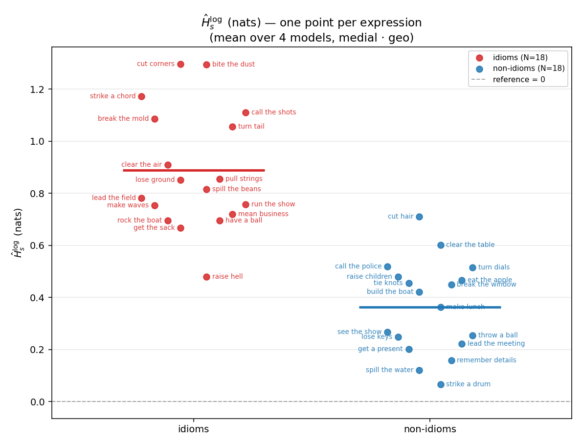
Log-space synergy \(H_s^{\log}\)
The average surprisal reduction the phrase achieves over its best component word, with
non-synergistic contexts contributing 0. Always finite; increases with synergy. A signed variant,
\(\mathbb E_{c\sim p}[s(c)]\) (stored as h_s_log_signed_idiom), can go negative when
non-synergistic contexts dominate. \(H_s^{\log}\) is not an ad-hoc replacement for
\(H_s\): per context the two carry the same information through an exact
change of variables (next page), and \(H_s^{\log}\) satisfies an exact identity:
The exact identity \(H_u = H(p) + H_s^{\log}\)
Lemma (pointwise). For \(a, b > 0\): \(\min\{a,b\}\) is the smaller value and \(-\log\) is strictly decreasing, so the log of the smaller value is the larger surprisal: \(-\log\min\{a,b\} = \max(-\log a,\, -\log b)\). \(\;\blacksquare\)
Theorem. Apply the Lemma with \(a = p(c)\), \(b = m(c)\), then the elementary identity \(\max(\alpha,\beta) = \alpha + \max(0,\, \beta-\alpha)\) with \(\alpha = -\log p(c)\), \(\beta = -\log m(c)\). This gives, for every context \(c\) (a deterministic, pointwise statement):
Because it holds pointwise, applying \(\mathbb E_{c\sim p}[\cdot]\) to both sides gives the population identity \(H_u = H(p) + H_s^{\log}\), and applying the sample mean \(\frac1N\sum_i[\cdot]\) gives the same identity for the estimators:
The split is exact at both the population and the estimate level (verified in the data to \(\sim 10^{-15}\)). Corollary, dividing by \(\hat H(p)\):
So the headline ratio is exactly 1 plus the synergy estimator rescaled by the
base-entropy estimator (\(\hat r_s^{\log}\) is stored as ratio_s_log_idiom). It is therefore
not independent of \(\hat H(p)\) — which is exactly what the analysis
page untangles.
Regularized synergy entropy \(H_s^{\mathrm{reg}}\)
\(H_s\) with the excess floored at \(\varepsilon p\): a
non-synergistic context contributes \(-\log p(c) + \log\frac1\varepsilon\) — large but finite — instead of
\(+\infty\). Decreases with synergy; continuous in the number of non-synergistic contexts. Reported as
h_s_reg_idiom with ratio ratio_s_reg_idiom (\(\ge 1\)).
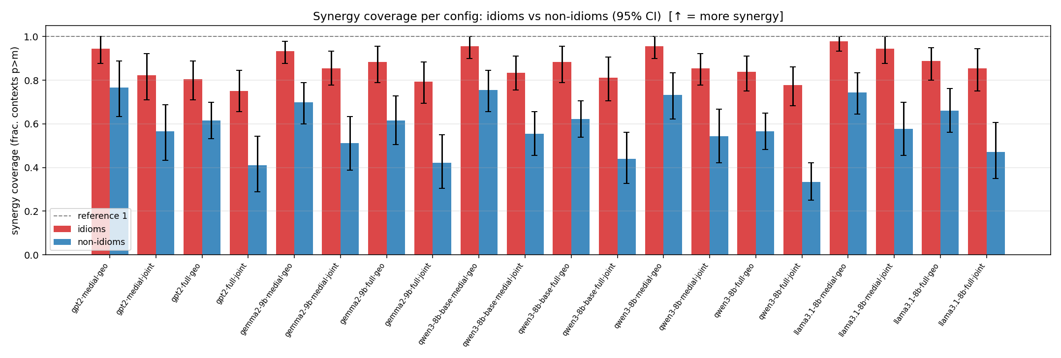
Synergistic fraction \(f_{\mathrm{syn}}\)
The probability that a context is synergistic, estimated by the observed fraction.
\(\hat f_{\mathrm{syn}} = 1\) is exactly the condition for \(\hat H_s\) to be finite. Stored as
syn_frac_idiom.
Quick reference: ranges, directions, JSON keys
\(H(p), H_u, H_s, H_s^{\mathrm{reg}}\) are expectations of surprisals \(-\log(\cdot)\), so they decrease as their argument grows; \(H_s^{\log}\) and \(f_{\mathrm{syn}}\) increase with synergy.
| metric | JSON key | range | direction | one-liner |
|---|---|---|---|---|
| \(H(p)\) | entropy_idiom |
\(\ge 0\) | smaller = more concentrated | spread of the phrase over its contexts |
| \(H_u/H(p)\) | ratio_u_idiom |
\(\ge 1\) | increases with synergy | primary comparison: concentration beyond the best component word |
| \(H_u\) | h_u_idiom |
\(\ge H(p)\) | read via the ratio | surprisal of the atom-best cover |
| \(f_{\mathrm{syn}}\) | syn_frac_idiom |
\([0,1]\) | increases with synergy | estimated \(P(\text{context is synergistic})\) |
| \(H_s^{\log}\) (and \(/H\)) | h_s_log_idiom, ratio_s_log_idiom |
\(\ge 0\) | increases with synergy | mean surprisal reduction vs the best word; \(= H_u - H(p)\) exactly |
| signed \(\mathbb E[s]\) | h_s_log_signed_idiom |
\(\mathbb R\) | increases with synergy | signed mean log-synergy; negative when non-synergistic slots dominate |
| \(H_s^{\mathrm{reg}}\) (and \(/H\)) | h_s_reg_idiom, ratio_s_reg_idiom |
\(> H(p)\) / \(> 1\) | decreases with synergy | \(H_s\) with the excess floored at \(\varepsilon p\); finite, continuous |
| \(H_s\) (and \(/H\)) | h_s_idiom, ratio_s_idiom |
\(> H(p)\) or \(+\infty\) | decreases with synergy | surprisal of the excess; \(+\infty\) iff some context is non-synergistic |
Each phrase's JSON row also carries bound_ok (the
AM–GM bound check), the sample counts
n_idiom_ctx/n_head_ctx/n_non_ctx, and the raw per-context vectors
p_ctx/q_ctx/r_ctx, so every metric can be recomputed offline.
Hs vs Hslog, and the AM–GM bound
Notation as on the profiles and entropies pages: contexts are an i.i.d. sample \(c_1,\dots,c_N\sim p\), and per context \(U(c)=\min\{p(c),m(c)\}\), \(S(c)=\max\{0,\,p(c)-m(c)\}\), \(s(c)=\log p(c)-\log m(c)\), with the pointwise additive split \(U(c)+S(c)=p(c)\). The two synergy entropies are the population expectations
with MC estimators \(\hat H_s,\ \hat H_s^{\log}\) (sample means over the observed contexts). \(H_s\) is the original, principled definition — the surprisal of the synergistic excess, the quantity for which the split is additive. \(H_s^{\log}\) is not a separate ad-hoc construction: per context it is the same information as \(H_s\), connected by an exact change of variables, as follows.
Pointwise change of variables: \(-\log S(c) = -\log p(c) + \varphi(s(c))\)
On a synergistic context (\(s(c)>0\)) the excess factorizes against the phrase's own score:
This is a deterministic, pointwise identity, so the sample mean (and identically \(\mathbb{E}_{c\sim p}\)) preserves it:
(verified in the sweep data to machine precision). \(\varphi\) is strictly decreasing, with \(\varphi(s)\to+\infty\) as \(s\downarrow 0\) and \(\varphi(s)\approx e^{-s}\to 0\) as \(s\to\infty\). So per context, \(\hat H_s^{\log}\) averages \(s\) itself while \(\hat H_s\) averages the strictly decreasing transform \(\varphi(s)\) of the same variable, plus the base surprisal. This accounts for every observed behavior of \(H_s\): (i) its direction is inverted (more synergy ⇒ smaller \(\hat H_s\)); (ii) it has a pole at zero synergy (one context with \(s\le 0\) ⇒ \(\hat H_s=+\infty\)); (iii) it mixes concentration with synergy (the \(\hat H(p)\) offset), whereas \(\hat H_s^{\log}=\hat H_u-\hat H(p)\) isolates the synergy term. Per context the map is one-to-one; per phrase the two sample means are not deterministic functions of each other (they average different transforms), but for a phrase whose contexts share a common log-synergy \(s\) the relation is exact: \(\hat H_s = \hat H(p) + \varphi(\hat H_s^{\log})\).
The split at the expectation level
Taking expectations of \(U+S=p\) (linearity — no convexity is involved):
and since all three means lie in \((0,1]\) (so \(ab\le a+b\)),
The split is exact in linear space. The entropies, however, average \(-\log\) pointwise, which tightens this into a quantitative bound:
The AM–GM bound: \(H_u + H_s \ \ge\ 2H(p) + 2\log 2 \ \ge\ H(p)\)
For every context, \(U(c),S(c)\ge 0\) and \(U(c)+S(c)=p(c)\), so by AM–GM
with equality iff \(U(c)=S(c)\), i.e. \(m(c)=p(c)/2\), i.e. \(s(c)=\log 2\). The inequality is pointwise, so both the population expectation and the sample mean preserve it:
the last step because \(\hat H(p)\ge 0\); identically for the population quantities. This is
the bound_ok check in main.py; it holds for every phrase in every config (trivially
when \(\hat H_s=+\infty\)). In particular the two surprisal terms do not sum to \(H(p)\) — the
additive split lives in linear space (previous subsection), not in surprisal space. Substituting the
identity \(\hat H_u = \hat H(p) + \hat H_s^{\log}\) gives the pure
synergy form of the same bound,
whose pointwise version is the one-dimensional statement \(s + \varphi(s) \ge 2\log 2\), minimized exactly at \(s=\log 2\) (left panel below).
Picture and data
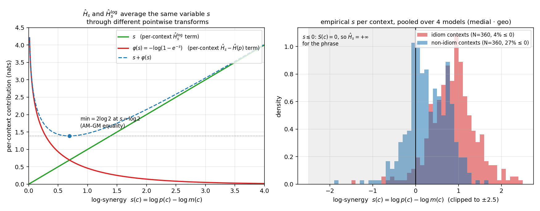
Where \(\hat H_s\) is finite
\(\hat H_s\) is finite exactly when every observed context is synergistic (\(\hat f_{\mathrm{syn}}=1\)). In the medial · geo configs this holds for most idiom phrases but few non-idiom phrases — itself a comparison in the expected direction:
| config (medial · geo) | idiom phrases with finite \(\hat H_s\) | non-idiom phrases with finite \(\hat H_s\) |
|---|---|---|
| gpt2 | 15/18 | 8/18 |
| gemma2-9b | 13/18 | 3/18 |
| qwen3-8b-base | 15/18 | 4/18 |
| qwen3-8b | 15/18 | 6/18 |
| llama3.1-8b | 17/18 | 5/18 |
Practice. Both quantities are reported throughout. \(\hat H_s\) is the principled surprisal of the excess and the quantity entering the AM–GM bound; on the (mostly idiom) phrases where it is finite it is directly comparable. \(\hat H_s^{\log} = \hat H_u - \hat H(p)\) carries the same per-context information through a finite, increasing transform, and therefore supports phrase-level comparison when some contexts are non-synergistic. \(\hat H_s^{\mathrm{reg}}\) keeps \(H_s\)'s form with the excess floored at \(\varepsilon p\); \(\hat f_{\mathrm{syn}}\) estimates \(P_{c\sim p}(S(c)>0)\).
Is the ratio just H(p)?
\(\hat H(p)\) differs sharply between idioms and non-idioms (idioms lower), and \(\hat H(p)\) sits in the denominator of the headline ratio. By the exact identity \(\hat H_u = \hat H(p) + \hat H_s^{\log}\),
so before claiming idioms have more synergy, we must rule out that "idioms have higher \(\hat H_u/\hat H(p)\)" is merely "idioms have smaller \(\hat H(p)\)". This page states the confound, develops two complementary tests, and reports the numbers.
The confound, stated precisely
Let \(D=1\) for idioms, \(0\) for non-idioms. Empirically \(D\) shifts both \(\hat H(p)\) (down) and \(\hat H_u/\hat H(p)\) (up). By the identity, a group difference in the ratio can come from (i) a larger numerator \(\hat H_s^{\log}\), or (ii) a smaller denominator \(\hat H(p)\), or both. The substantive, theory-backed claim is (i) — the idiom concentrates beyond what its best word predicts. We must isolate (i) from (ii).
Why dividing is not controlling
Forming the ratio does not remove the \(\hat H(p)\) effect. "Controlling for \(\hat H(p)\)" means estimating the group effect at a fixed value of \(\hat H(p)\) — a conditional (partial) effect. A ratio instead rescales by \(\hat H(p)\): for equal absolute synergy, the phrase with smaller \(\hat H(p)\) gets a larger ratio, so the ratio can move purely because the denominator shrank. We therefore test the numerator directly, two ways.
Method A — ANCOVA: the partial effect at fixed H(p)
Let phrase \(j\) have estimators \(S_j := \hat H_s^{\log}\) and \(H_j := \hat H(p)\), and \(D_j\in\{0,1\}\). Across the \(2{\times}18\) phrases fit by ordinary least squares:
\(\beta\) is the idiom–nonidiom difference in synergy holding \(H(p)\) fixed. We test \(H_0:\beta=0\) with \(t=\hat\beta/\operatorname{se}(\hat\beta)\), \(\mathrm{df}=n-3\), where \(\operatorname{se}=\sqrt{\bigl[\hat\sigma^2 (X^{\top}X)^{-1}\bigr]_{\beta\beta}}\) and \(\hat\sigma^2=\mathrm{RSS}/\mathrm{df}\). Comparing \(\hat\beta\) to the uncontrolled slope from \(S=\alpha+\beta D\) shows how much of the raw synergy gap \(H(p)\) accounts for. The pooled fit adds model fixed effects (dummies).
Method B — exact decomposition of the ratio gap
With group means \(\bar S_i,\bar S_n,\bar H_i,\bar H_n\), add and subtract \(\bar S_n/\bar H_i\):
The first term is the gap that would remain if both groups shared idioms' \(H(p)\); the second is the gap that would remain if both groups shared non-idioms' synergy. Each term's share of \(\Delta R\) is the % of the ratio gap that source explains.
Caveat — H(p) is partly a mediator
\(H_s^{\log}\) and \(H(p)\) are negatively correlated (more concentrated ⇒ more synergy; see the correlation column in the results below). If low \(H(p)\) is itself a consequence of idiomaticity, then \(H(p)\) is a mediator, not a pure confounder, and the ANCOVA \(\beta\) under-states the total idiom effect. So the controlled \(\beta\) is a conservative lower bound; the true effect lies between it and the uncontrolled slope.
Results — decomposition of the ratio gap (Method B)
Per-config (medial · geo) and pooled across the five models. All entries are the
per-phrase MC estimators (group means \(\bar S,\bar H\) are over
phrases). Rerun for any mode/reduction with
python code/confound_check.py --mode MODE --red RED.
Per-config group means, the ratio gap ΔR, and the share carried by the synergy numerator vs the H(p) denominator.
| config | H(p) idiom | H(p) non | Hslog idiom | Hslog non | ratio_u idiom | ratio_u non | ΔR | synergy % | H(p) % |
|---|---|---|---|---|---|---|---|---|---|
| gpt2 | 4.405 | 4.733 | 0.597 | 0.268 | 1.143 | 1.059 | +0.0790 | 95% | 5% |
| gemma2-9b | 4.388 | 5.180 | 1.016 | 0.446 | 1.240 | 1.091 | +0.1454 | 89% | 11% |
| qwen3-8b-base | 4.083 | 4.608 | 0.853 | 0.341 | 1.217 | 1.076 | +0.1349 | 93% | 7% |
| qwen3-8b | 4.462 | 5.031 | 0.867 | 0.348 | 1.201 | 1.072 | +0.1251 | 93% | 7% |
| llama3.1-8b | 4.047 | 4.651 | 0.818 | 0.313 | 1.207 | 1.070 | +0.1348 | 93% | 7% |
| POOLED (5 models, +model FE) | 4.277 | 4.840 | 0.830 | 0.343 | 1.202 | 1.074 | +0.1232 | 92% | 8% |
Results — ANCOVA on Hslog (Method A)
Idiom coefficient β without and with H(p) as a covariate, the % the effect shrinks when H(p) is controlled, the H(p) slope γ, and the Hslog–H(p) correlation. β stays large and significant at fixed H(p).
| config | β uncontrolled (S ~ D) | β controlled (S ~ D + H(p)) | p (controlled) | shrink | γ = H(p) coef | corr(Hslog, H(p)) |
|---|---|---|---|---|---|---|
| gpt2 | +0.330 | +0.276 | 2e-04 | +16% | -0.164 (p=0.004) | -0.52 |
| gemma2-9b | +0.570 | +0.532 | 4e-06 | +7% | -0.047 (p=0.359) | -0.41 |
| qwen3-8b-base | +0.512 | +0.446 | 7e-07 | +13% | -0.127 (p=0.025) | -0.52 |
| qwen3-8b | +0.519 | +0.431 | 3e-06 | +17% | -0.154 (p=0.011) | -0.57 |
| llama3.1-8b | +0.505 | +0.429 | 1e-07 | +15% | -0.126 (p=0.019) | -0.59 |
| POOLED (5 models, +model FE) | +0.487 | +0.422 | 9e-26 | +13% | -0.115 (p=2e-06) | -0.44 |
Verdict
Practice. Report the synergy as the additive Hslog = Hu − H(p) and test it with the ANCOVA above (or its non-finite-safe siblings), rather than treating Hu/H(p) as if it controlled for H(p). The ratio is a fine convenience index, but it conflates "more synergy" with "lower base entropy". Rerun with python code/confound_check.py --mode MODE --red RED.
Aggregate plots (across all configs)
Cross-model views combining the per-config results. Metric definitions: entropies & estimators. Click any figure to zoom.
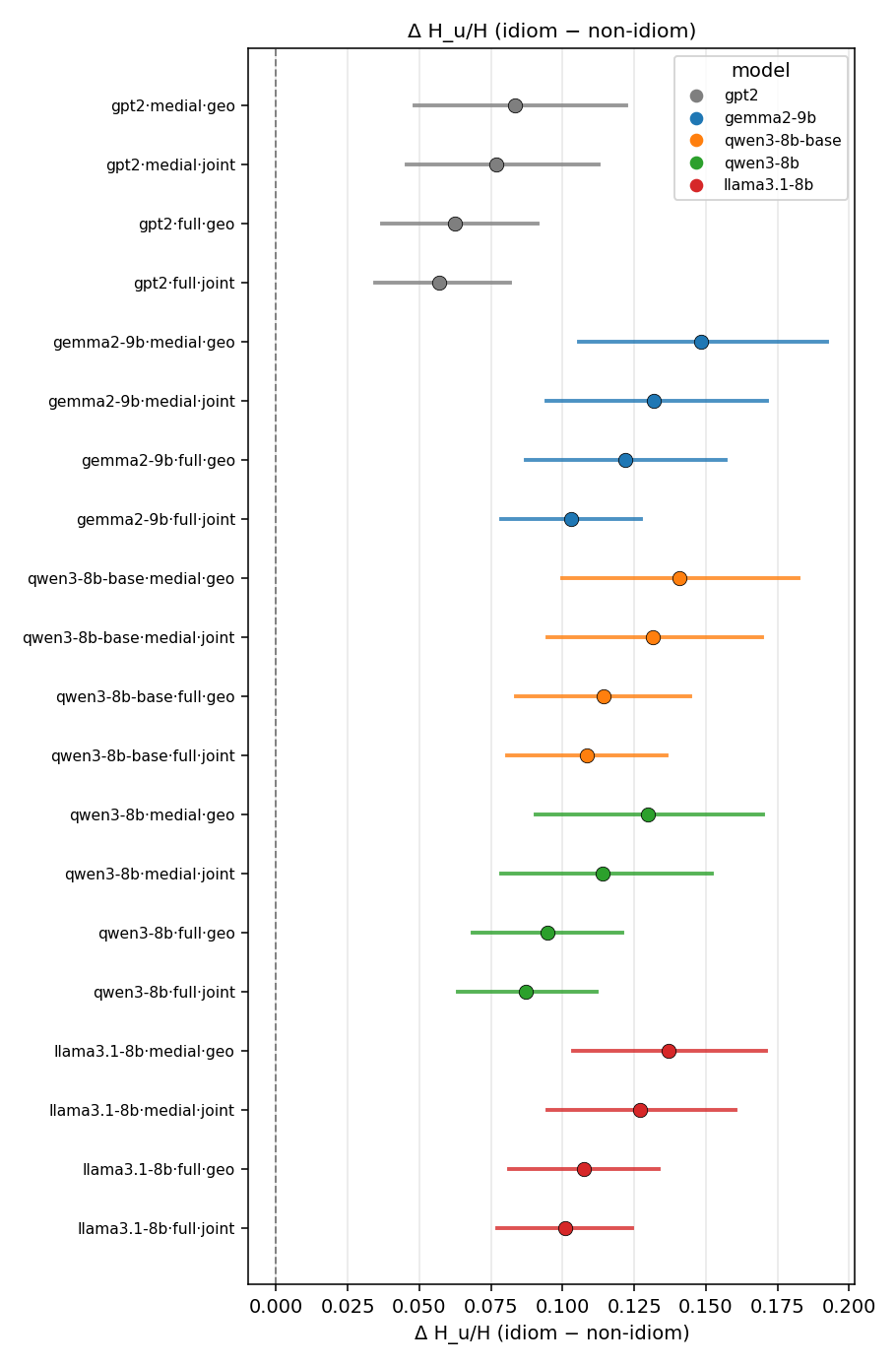
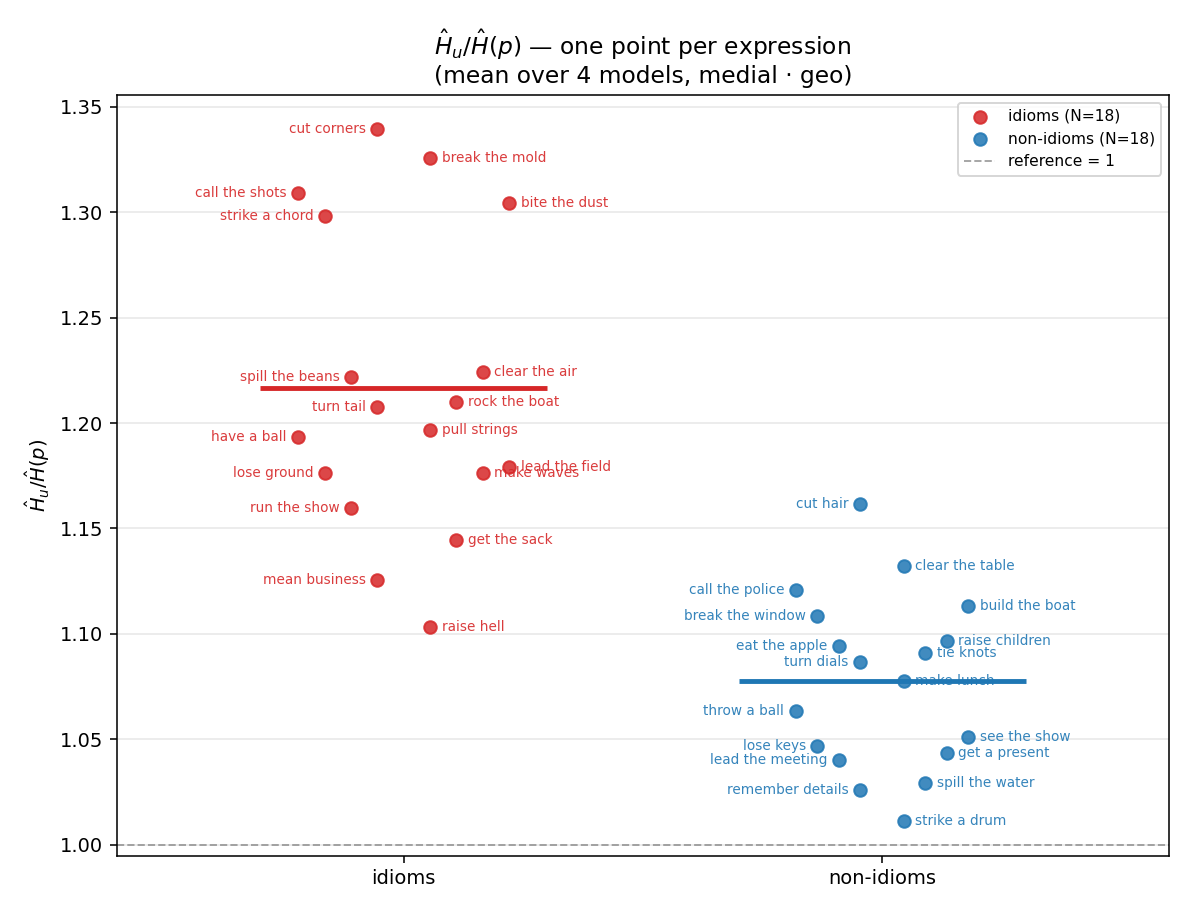
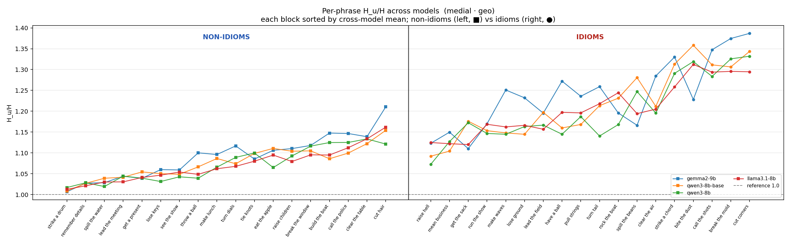
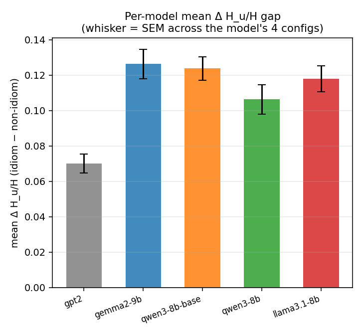
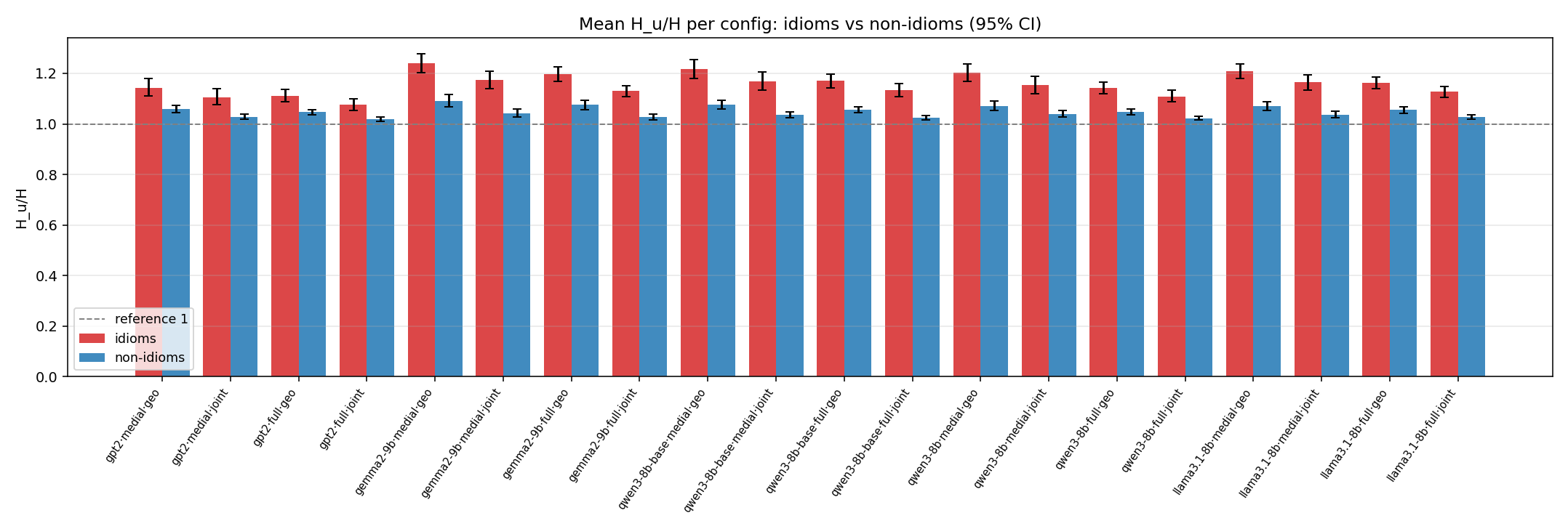
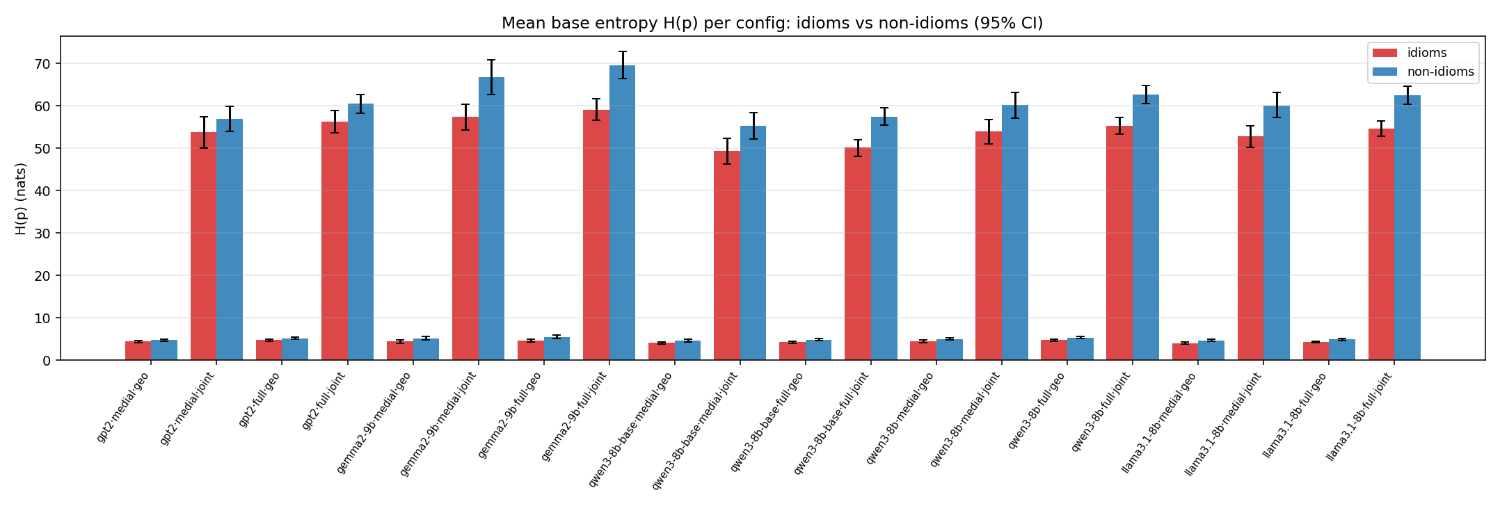
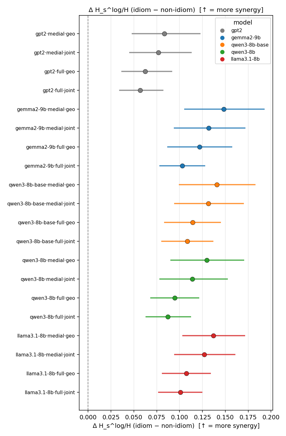
Bootstrap summary tables
All entries are per-phrase Monte-Carlo estimates of the corresponding population quantities. Each table gives the per-config mean for idioms and non-idioms (with finite-phrase count fin/N), and the idiom−nonidiom gap with a 20k-resample independent bootstrap 95% CI. Rows whose CI excludes 0 are shaded and marked ✓.
\(\hat H_u / \hat H(p)\)
unique-information ratio, ≥ 1; equals 1 iff no observed context is synergistic. Primary comparison; increases with synergy — definition
| model | mode | reduction | idiom mean (fin/N) | non-idiom mean (fin/N) | Δ idiom−nonidiom | 95% CI | sig |
|---|---|---|---|---|---|---|---|
| gpt2 | medial | geo | 1.143 (18/18) | 1.059 (18/18) | 0.084 | [0.048, 0.122] | ✓ |
| gpt2 | medial | joint | 1.105 (18/18) | 1.028 (18/18) | 0.077 | [0.046, 0.113] | ✓ |
| gpt2 | full | geo | 1.110 (18/18) | 1.047 (18/18) | 0.063 | [0.037, 0.091] | ✓ |
| gpt2 | full | joint | 1.075 (18/18) | 1.018 (18/18) | 0.057 | [0.034, 0.082] | ✓ |
| gemma2-9b | medial | geo | 1.240 (18/18) | 1.091 (18/18) | 0.148 | [0.106, 0.192] | ✓ |
| gemma2-9b | medial | joint | 1.173 (18/18) | 1.041 (18/18) | 0.132 | [0.095, 0.171] | ✓ |
| gemma2-9b | full | geo | 1.197 (18/18) | 1.075 (18/18) | 0.122 | [0.087, 0.157] | ✓ |
| gemma2-9b | full | joint | 1.130 (18/18) | 1.027 (18/18) | 0.103 | [0.079, 0.127] | ✓ |
| qwen3-8b-base | medial | geo | 1.217 (18/18) | 1.076 (18/18) | 0.141 | [0.100, 0.182] | ✓ |
| qwen3-8b-base | medial | joint | 1.168 (18/18) | 1.037 (18/18) | 0.132 | [0.095, 0.170] | ✓ |
| qwen3-8b-base | full | geo | 1.170 (18/18) | 1.056 (18/18) | 0.114 | [0.084, 0.145] | ✓ |
| qwen3-8b-base | full | joint | 1.134 (18/18) | 1.025 (18/18) | 0.108 | [0.081, 0.136] | ✓ |
| qwen3-8b | medial | geo | 1.201 (18/18) | 1.072 (18/18) | 0.130 | [0.091, 0.170] | ✓ |
| qwen3-8b | medial | joint | 1.153 (18/18) | 1.039 (18/18) | 0.114 | [0.079, 0.152] | ✓ |
| qwen3-8b | full | geo | 1.142 (18/18) | 1.047 (18/18) | 0.095 | [0.069, 0.121] | ✓ |
| qwen3-8b | full | joint | 1.109 (18/18) | 1.022 (18/18) | 0.087 | [0.064, 0.112] | ✓ |
| llama3.1-8b | medial | geo | 1.207 (18/18) | 1.070 (18/18) | 0.137 | [0.104, 0.171] | ✓ |
| llama3.1-8b | medial | joint | 1.164 (18/18) | 1.037 (18/18) | 0.127 | [0.095, 0.160] | ✓ |
| llama3.1-8b | full | geo | 1.163 (18/18) | 1.055 (18/18) | 0.108 | [0.081, 0.134] | ✓ |
| llama3.1-8b | full | joint | 1.127 (18/18) | 1.027 (18/18) | 0.101 | [0.077, 0.124] | ✓ |
\(\hat H_u\)
unique-information entropy (nats); ≥ \(\hat H(p)\) by construction — read via the ratio — definition
| model | mode | reduction | idiom mean (fin/N) | non-idiom mean (fin/N) | Δ idiom−nonidiom | 95% CI | sig |
|---|---|---|---|---|---|---|---|
| gpt2 | medial | geo | 5.003 (18/18) | 5.001 (18/18) | 0.002 | [-0.352, 0.355] | |
| gpt2 | medial | joint | 59.207 (18/18) | 58.475 (18/18) | 0.732 | [-4.048, 5.556] | |
| gpt2 | full | geo | 5.255 (18/18) | 5.355 (18/18) | -0.100 | [-0.412, 0.204] | |
| gpt2 | full | joint | 60.424 (18/18) | 61.565 (18/18) | -1.141 | [-4.379, 2.284] | |
| gemma2-9b | medial | geo | 5.404 (18/18) | 5.627 (18/18) | -0.222 | [-0.791, 0.346] | |
| gemma2-9b | medial | joint | 67.242 (18/18) | 69.420 (18/18) | -2.179 | [-7.442, 2.991] | |
| gemma2-9b | full | geo | 5.540 (18/18) | 5.896 (18/18) | -0.357 | [-0.832, 0.110] | |
| gemma2-9b | full | joint | 66.644 (18/18) | 71.386 (18/18) | -4.741 | [-8.562, -0.865] | ✓ |
| qwen3-8b-base | medial | geo | 4.935 (18/18) | 4.948 (18/18) | -0.013 | [-0.392, 0.367] | |
| qwen3-8b-base | medial | joint | 57.427 (18/18) | 57.338 (18/18) | 0.089 | [-4.414, 4.643] | |
| qwen3-8b-base | full | geo | 4.981 (18/18) | 5.130 (18/18) | -0.149 | [-0.457, 0.155] | |
| qwen3-8b-base | full | joint | 56.744 (18/18) | 58.946 (18/18) | -2.202 | [-4.842, 0.431] | |
| qwen3-8b | medial | geo | 5.329 (18/18) | 5.379 (18/18) | -0.050 | [-0.412, 0.312] | |
| qwen3-8b | medial | joint | 61.997 (18/18) | 62.510 (18/18) | -0.513 | [-4.777, 3.839] | |
| qwen3-8b | full | geo | 5.370 (18/18) | 5.564 (18/18) | -0.194 | [-0.500, 0.107] | |
| qwen3-8b | full | joint | 61.273 (18/18) | 64.110 (18/18) | -2.837 | [-5.511, -0.111] | ✓ |
| llama3.1-8b | medial | geo | 4.865 (18/18) | 4.964 (18/18) | -0.099 | [-0.438, 0.241] | |
| llama3.1-8b | medial | joint | 61.434 (18/18) | 62.319 (18/18) | -0.885 | [-4.984, 3.254] | |
| llama3.1-8b | full | geo | 4.979 (18/18) | 5.153 (18/18) | -0.174 | [-0.458, 0.110] | |
| llama3.1-8b | full | joint | 61.542 (18/18) | 64.133 (18/18) | -2.591 | [-5.304, 0.151] |
\(\hat H(p)\)
base entropy (nats); smaller = phrase more concentrated over its contexts — definition
| model | mode | reduction | idiom mean (fin/N) | non-idiom mean (fin/N) | Δ idiom−nonidiom | 95% CI | sig |
|---|---|---|---|---|---|---|---|
| gpt2 | medial | geo | 4.405 (18/18) | 4.733 (18/18) | -0.327 | [-0.728, 0.068] | |
| gpt2 | medial | joint | 53.784 (18/18) | 56.898 (18/18) | -3.114 | [-7.793, 1.533] | |
| gpt2 | full | geo | 4.748 (18/18) | 5.124 (18/18) | -0.376 | [-0.723, -0.043] | ✓ |
| gpt2 | full | joint | 56.326 (18/18) | 60.490 (18/18) | -4.164 | [-7.626, -0.648] | ✓ |
| gemma2-9b | medial | geo | 4.388 (18/18) | 5.180 (18/18) | -0.792 | [-1.358, -0.227] | ✓ |
| gemma2-9b | medial | joint | 57.510 (18/18) | 66.768 (18/18) | -9.258 | [-14.355, -4.175] | ✓ |
| gemma2-9b | full | geo | 4.648 (18/18) | 5.507 (18/18) | -0.860 | [-1.353, -0.373] | ✓ |
| gemma2-9b | full | joint | 59.119 (18/18) | 69.592 (18/18) | -10.473 | [-14.544, -6.382] | ✓ |
| qwen3-8b-base | medial | geo | 4.083 (18/18) | 4.608 (18/18) | -0.525 | [-0.932, -0.113] | ✓ |
| qwen3-8b-base | medial | joint | 49.327 (18/18) | 55.334 (18/18) | -6.007 | [-10.345, -1.712] | ✓ |
| qwen3-8b-base | full | geo | 4.274 (18/18) | 4.868 (18/18) | -0.593 | [-0.936, -0.254] | ✓ |
| qwen3-8b-base | full | joint | 50.181 (18/18) | 57.521 (18/18) | -7.340 | [-10.174, -4.578] | ✓ |
| qwen3-8b | medial | geo | 4.462 (18/18) | 5.031 (18/18) | -0.569 | [-0.967, -0.165] | ✓ |
| qwen3-8b | medial | joint | 53.941 (18/18) | 60.211 (18/18) | -6.270 | [-10.398, -2.075] | ✓ |
| qwen3-8b | full | geo | 4.717 (18/18) | 5.320 (18/18) | -0.603 | [-0.944, -0.267] | ✓ |
| qwen3-8b | full | joint | 55.345 (18/18) | 62.749 (18/18) | -7.404 | [-10.265, -4.538] | ✓ |
| llama3.1-8b | medial | geo | 4.047 (18/18) | 4.651 (18/18) | -0.604 | [-0.979, -0.235] | ✓ |
| llama3.1-8b | medial | joint | 52.850 (18/18) | 60.144 (18/18) | -7.294 | [-11.182, -3.499] | ✓ |
| llama3.1-8b | full | geo | 4.293 (18/18) | 4.894 (18/18) | -0.601 | [-0.916, -0.294] | ✓ |
| llama3.1-8b | full | joint | 54.666 (18/18) | 62.505 (18/18) | -7.839 | [-10.650, -5.073] | ✓ |
\(\hat H_s\)
synergy entropy (nats): mean surprisal of the excess \(S(c)=\max\{0,p-m\}\); decreases with synergy; finite iff every context is synergistic (the fin/N column counts such phrases) — definition, relationship to \(\hat H_s^{\log}\)
| model | mode | reduction | idiom mean (fin/N) | non-idiom mean (fin/N) | Δ idiom−nonidiom | 95% CI | sig |
|---|---|---|---|---|---|---|---|
| gpt2 | medial | geo | 5.326 (15/18) | 5.892 (8/18) | -0.566 | [-1.133, 0.019] | |
| gpt2 | medial | joint | 54.443 (10/18) | 54.944 (2/18) | -0.501 | [-6.746, 5.519] | |
| gpt2 | full | geo | 5.019 (5/18) | 5.895 (1/18) | -0.876 | [-1.134, -0.686] | ✓ |
| gpt2 | full | joint | 52.454 (4/18) | 56.005 (2/18) | -3.550 | [-10.748, 3.419] | |
| gemma2-9b | medial | geo | 4.882 (13/18) | 5.653 (3/18) | -0.771 | [-1.825, 0.116] | |
| gemma2-9b | medial | joint | 57.353 (10/18) | 57.287 (1/18) | 0.066 | [-3.629, 3.862] | |
| gemma2-9b | full | geo | 4.871 (9/18) | 5.433 (1/18) | -0.562 | [-0.817, -0.283] | ✓ |
| gemma2-9b | full | joint | 59.718 (3/18) | 59.138 (1/18) | 0.580 | [-2.463, 5.771] | |
| qwen3-8b-base | medial | geo | 4.856 (15/18) | 5.746 (4/18) | -0.890 | [-1.497, -0.258] | ✓ |
| qwen3-8b-base | medial | joint | 49.063 (8/18) | — (0/18) | — | — | |
| qwen3-8b-base | full | geo | 4.774 (9/18) | — (0/18) | — | — | |
| qwen3-8b-base | full | joint | 47.830 (5/18) | — (0/18) | — | — | |
| qwen3-8b | medial | geo | 5.162 (15/18) | 5.769 (6/18) | -0.607 | [-1.159, -0.077] | ✓ |
| qwen3-8b | medial | joint | 52.503 (9/18) | 62.247 (1/18) | -9.744 | [-12.984, -6.662] | ✓ |
| qwen3-8b | full | geo | 5.089 (4/18) | — (0/18) | — | — | |
| qwen3-8b | full | joint | 49.996 (2/18) | — (0/18) | — | — | |
| llama3.1-8b | medial | geo | 4.739 (17/18) | 5.582 (5/18) | -0.844 | [-1.472, -0.242] | ✓ |
| llama3.1-8b | medial | joint | 52.826 (15/18) | 57.031 (2/18) | -4.205 | [-9.214, 0.812] | |
| llama3.1-8b | full | geo | 4.960 (8/18) | 5.424 (1/18) | -0.465 | [-0.829, -0.042] | ✓ |
| llama3.1-8b | full | joint | 53.727 (8/18) | 58.867 (2/18) | -5.140 | [-8.788, -1.453] | ✓ |
\(\hat H_s / \hat H(p)\)
synergy-entropy ratio; finite on the same phrases as \(\hat H_s\) — definition
| model | mode | reduction | idiom mean (fin/N) | non-idiom mean (fin/N) | Δ idiom−nonidiom | 95% CI | sig |
|---|---|---|---|---|---|---|---|
| gpt2 | medial | geo | 1.211 (15/18) | 1.352 (8/18) | -0.141 | [-0.213, -0.069] | ✓ |
| gpt2 | medial | joint | 1.001 (10/18) | 1.004 (2/18) | -0.003 | [-0.008, 0.001] | |
| gpt2 | full | geo | 1.194 (5/18) | 1.382 (1/18) | -0.188 | [-0.239, -0.152] | ✓ |
| gpt2 | full | joint | 1.000 (4/18) | 1.004 (2/18) | -0.004 | [-0.005, -0.002] | ✓ |
| gemma2-9b | medial | geo | 1.124 (13/18) | 1.302 (3/18) | -0.178 | [-0.414, 0.006] | |
| gemma2-9b | medial | joint | 1.000 (10/18) | 1.000 (1/18) | 0.000 | [-0.000, 0.001] | |
| gemma2-9b | full | geo | 1.148 (9/18) | 1.214 (1/18) | -0.066 | [-0.092, -0.040] | ✓ |
| gemma2-9b | full | joint | 1.000 (3/18) | 1.001 (1/18) | -0.001 | [-0.001, -0.001] | ✓ |
| qwen3-8b-base | medial | geo | 1.177 (15/18) | 1.354 (4/18) | -0.177 | [-0.329, -0.062] | ✓ |
| qwen3-8b-base | medial | joint | 1.001 (8/18) | — (0/18) | — | — | |
| qwen3-8b-base | full | geo | 1.198 (9/18) | — (0/18) | — | — | |
| qwen3-8b-base | full | joint | 1.001 (5/18) | — (0/18) | — | — | |
| qwen3-8b | medial | geo | 1.153 (15/18) | 1.256 (6/18) | -0.103 | [-0.151, -0.054] | ✓ |
| qwen3-8b | medial | joint | 1.002 (9/18) | 1.002 (1/18) | -0.001 | [-0.002, 0.001] | |
| qwen3-8b | full | geo | 1.203 (4/18) | — (0/18) | — | — | |
| qwen3-8b | full | joint | 1.001 (2/18) | — (0/18) | — | — | |
| llama3.1-8b | medial | geo | 1.170 (17/18) | 1.316 (5/18) | -0.146 | [-0.283, -0.039] | ✓ |
| llama3.1-8b | medial | joint | 1.001 (15/18) | 1.001 (2/18) | 0.000 | [-0.000, 0.001] | |
| llama3.1-8b | full | geo | 1.196 (8/18) | 1.321 (1/18) | -0.124 | [-0.159, -0.092] | ✓ |
| llama3.1-8b | full | joint | 1.001 (8/18) | 1.003 (2/18) | -0.002 | [-0.005, 0.000] |
\(\hat H_s^{\log}\)
log-space synergy (nats) \(= \hat H_u - \hat H(p)\), exactly; always finite; increases with synergy — definition, the identity
| model | mode | reduction | idiom mean (fin/N) | non-idiom mean (fin/N) | Δ idiom−nonidiom | 95% CI | sig |
|---|---|---|---|---|---|---|---|
| gpt2 | medial | geo | 0.597 (18/18) | 0.268 (18/18) | 0.330 | [0.200, 0.468] | ✓ |
| gpt2 | medial | joint | 5.423 (18/18) | 1.577 (18/18) | 3.847 | [2.358, 5.395] | ✓ |
| gpt2 | full | geo | 0.507 (18/18) | 0.231 (18/18) | 0.276 | [0.168, 0.398] | ✓ |
| gpt2 | full | joint | 4.097 (18/18) | 1.074 (18/18) | 3.023 | [1.895, 4.223] | ✓ |
| gemma2-9b | medial | geo | 1.016 (18/18) | 0.446 (18/18) | 0.570 | [0.404, 0.737] | ✓ |
| gemma2-9b | medial | joint | 9.732 (18/18) | 2.653 (18/18) | 7.079 | [5.042, 9.162] | ✓ |
| gemma2-9b | full | geo | 0.892 (18/18) | 0.389 (18/18) | 0.503 | [0.360, 0.650] | ✓ |
| gemma2-9b | full | joint | 7.526 (18/18) | 1.794 (18/18) | 5.732 | [4.414, 7.031] | ✓ |
| qwen3-8b-base | medial | geo | 0.853 (18/18) | 0.341 (18/18) | 0.512 | [0.376, 0.651] | ✓ |
| qwen3-8b-base | medial | joint | 8.100 (18/18) | 2.004 (18/18) | 6.096 | [4.425, 7.808] | ✓ |
| qwen3-8b-base | full | geo | 0.707 (18/18) | 0.263 (18/18) | 0.444 | [0.334, 0.556] | ✓ |
| qwen3-8b-base | full | joint | 6.563 (18/18) | 1.425 (18/18) | 5.137 | [3.854, 6.416] | ✓ |
| qwen3-8b | medial | geo | 0.867 (18/18) | 0.348 (18/18) | 0.519 | [0.376, 0.662] | ✓ |
| qwen3-8b | medial | joint | 8.056 (18/18) | 2.299 (18/18) | 5.757 | [4.013, 7.577] | ✓ |
| qwen3-8b | full | geo | 0.653 (18/18) | 0.243 (18/18) | 0.410 | [0.302, 0.520] | ✓ |
| qwen3-8b | full | joint | 5.928 (18/18) | 1.361 (18/18) | 4.566 | [3.373, 5.789] | ✓ |
| llama3.1-8b | medial | geo | 0.818 (18/18) | 0.313 (18/18) | 0.505 | [0.390, 0.623] | ✓ |
| llama3.1-8b | medial | joint | 8.584 (18/18) | 2.175 (18/18) | 6.409 | [4.733, 8.116] | ✓ |
| llama3.1-8b | full | geo | 0.686 (18/18) | 0.259 (18/18) | 0.427 | [0.328, 0.530] | ✓ |
| llama3.1-8b | full | joint | 6.876 (18/18) | 1.628 (18/18) | 5.248 | [4.016, 6.479] | ✓ |
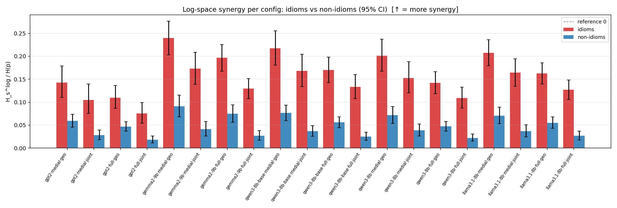
\(\hat H_s^{\log} / \hat H(p)\)
log-space synergy ratio \(\hat r_s^{\log} = \hat H_u/\hat H(p) - 1\); increases with synergy — definition
| model | mode | reduction | idiom mean (fin/N) | non-idiom mean (fin/N) | Δ idiom−nonidiom | 95% CI | sig |
|---|---|---|---|---|---|---|---|
| gpt2 | medial | geo | 0.143 (18/18) | 0.059 (18/18) | 0.084 | [0.048, 0.122] | ✓ |
| gpt2 | medial | joint | 0.105 (18/18) | 0.028 (18/18) | 0.077 | [0.046, 0.113] | ✓ |
| gpt2 | full | geo | 0.110 (18/18) | 0.047 (18/18) | 0.063 | [0.037, 0.091] | ✓ |
| gpt2 | full | joint | 0.075 (18/18) | 0.018 (18/18) | 0.057 | [0.034, 0.082] | ✓ |
| gemma2-9b | medial | geo | 0.240 (18/18) | 0.091 (18/18) | 0.148 | [0.106, 0.192] | ✓ |
| gemma2-9b | medial | joint | 0.173 (18/18) | 0.041 (18/18) | 0.132 | [0.095, 0.171] | ✓ |
| gemma2-9b | full | geo | 0.197 (18/18) | 0.075 (18/18) | 0.122 | [0.087, 0.157] | ✓ |
| gemma2-9b | full | joint | 0.130 (18/18) | 0.027 (18/18) | 0.103 | [0.079, 0.127] | ✓ |
| qwen3-8b-base | medial | geo | 0.217 (18/18) | 0.076 (18/18) | 0.141 | [0.100, 0.182] | ✓ |
| qwen3-8b-base | medial | joint | 0.168 (18/18) | 0.037 (18/18) | 0.132 | [0.095, 0.170] | ✓ |
| qwen3-8b-base | full | geo | 0.170 (18/18) | 0.056 (18/18) | 0.114 | [0.084, 0.145] | ✓ |
| qwen3-8b-base | full | joint | 0.134 (18/18) | 0.025 (18/18) | 0.108 | [0.081, 0.136] | ✓ |
| qwen3-8b | medial | geo | 0.201 (18/18) | 0.072 (18/18) | 0.130 | [0.091, 0.170] | ✓ |
| qwen3-8b | medial | joint | 0.153 (18/18) | 0.039 (18/18) | 0.114 | [0.079, 0.152] | ✓ |
| qwen3-8b | full | geo | 0.142 (18/18) | 0.047 (18/18) | 0.095 | [0.069, 0.121] | ✓ |
| qwen3-8b | full | joint | 0.109 (18/18) | 0.022 (18/18) | 0.087 | [0.064, 0.112] | ✓ |
| llama3.1-8b | medial | geo | 0.207 (18/18) | 0.070 (18/18) | 0.137 | [0.104, 0.171] | ✓ |
| llama3.1-8b | medial | joint | 0.164 (18/18) | 0.037 (18/18) | 0.127 | [0.095, 0.160] | ✓ |
| llama3.1-8b | full | geo | 0.163 (18/18) | 0.055 (18/18) | 0.108 | [0.081, 0.134] | ✓ |
| llama3.1-8b | full | joint | 0.127 (18/18) | 0.027 (18/18) | 0.101 | [0.077, 0.124] | ✓ |
\(\hat H_s^{\mathrm{reg}}\)
\(\hat H_s\) with the excess floored at \(\varepsilon p\) (\(\varepsilon=0.01\)); finite and continuous; decreases with synergy — definition
| model | mode | reduction | idiom mean (fin/N) | non-idiom mean (fin/N) | Δ idiom−nonidiom | 95% CI | sig |
|---|---|---|---|---|---|---|---|
| gpt2 | medial | geo | 5.577 (18/18) | 6.979 (18/18) | -1.401 | [-2.217, -0.628] | ✓ |
| gpt2 | medial | joint | 54.688 (18/18) | 59.067 (18/18) | -4.378 | [-9.102, 0.168] | |
| gpt2 | full | geo | 6.511 (18/18) | 7.884 (18/18) | -1.373 | [-2.109, -0.666] | ✓ |
| gpt2 | full | joint | 57.583 (18/18) | 63.359 (18/18) | -5.776 | [-9.450, -2.116] | ✓ |
| gemma2-9b | medial | geo | 5.199 (18/18) | 7.318 (18/18) | -2.119 | [-2.936, -1.310] | ✓ |
| gemma2-9b | medial | joint | 58.195 (18/18) | 69.151 (18/18) | -10.956 | [-16.106, -5.805] | ✓ |
| gemma2-9b | full | geo | 5.754 (18/18) | 7.903 (18/18) | -2.149 | [-3.012, -1.264] | ✓ |
| gemma2-9b | full | joint | 60.119 (18/18) | 72.350 (18/18) | -12.231 | [-16.562, -7.847] | ✓ |
| qwen3-8b-base | medial | geo | 4.971 (18/18) | 6.767 (18/18) | -1.796 | [-2.479, -1.123] | ✓ |
| qwen3-8b-base | medial | joint | 50.115 (18/18) | 57.523 (18/18) | -7.408 | [-11.787, -3.121] | ✓ |
| qwen3-8b-base | full | geo | 5.519 (18/18) | 7.481 (18/18) | -1.962 | [-2.647, -1.264] | ✓ |
| qwen3-8b-base | full | joint | 51.096 (18/18) | 60.236 (18/18) | -9.140 | [-12.221, -6.128] | ✓ |
| qwen3-8b | medial | geo | 5.333 (18/18) | 7.263 (18/18) | -1.930 | [-2.645, -1.207] | ✓ |
| qwen3-8b | medial | joint | 54.672 (18/18) | 62.461 (18/18) | -7.789 | [-11.858, -3.655] | ✓ |
| qwen3-8b | full | geo | 6.171 (18/18) | 8.137 (18/18) | -1.966 | [-2.650, -1.274] | ✓ |
| qwen3-8b | full | joint | 56.448 (18/18) | 65.905 (18/18) | -9.457 | [-12.559, -6.406] | ✓ |
| llama3.1-8b | medial | geo | 4.818 (18/18) | 6.855 (18/18) | -2.037 | [-2.665, -1.403] | ✓ |
| llama3.1-8b | medial | joint | 53.152 (18/18) | 62.212 (18/18) | -9.060 | [-13.007, -5.224] | ✓ |
| llama3.1-8b | full | geo | 5.510 (18/18) | 7.452 (18/18) | -1.941 | [-2.614, -1.261] | ✓ |
| llama3.1-8b | full | joint | 55.396 (18/18) | 65.059 (18/18) | -9.663 | [-12.739, -6.633] | ✓ |
\(\hat H_s^{\mathrm{reg}} / \hat H(p)\)
regularized synergy ratio (≥ 1); decreases with synergy — definition
| model | mode | reduction | idiom mean (fin/N) | non-idiom mean (fin/N) | Δ idiom−nonidiom | 95% CI | sig |
|---|---|---|---|---|---|---|---|
| gpt2 | medial | geo | 1.264 (18/18) | 1.468 (18/18) | -0.204 | [-0.298, -0.107] | ✓ |
| gpt2 | medial | joint | 1.017 (18/18) | 1.039 (18/18) | -0.022 | [-0.036, -0.008] | ✓ |
| gpt2 | full | geo | 1.365 (18/18) | 1.536 (18/18) | -0.171 | [-0.250, -0.089] | ✓ |
| gpt2 | full | joint | 1.022 (18/18) | 1.048 (18/18) | -0.026 | [-0.038, -0.013] | ✓ |
| gemma2-9b | medial | geo | 1.187 (18/18) | 1.416 (18/18) | -0.228 | [-0.312, -0.137] | ✓ |
| gemma2-9b | medial | joint | 1.012 (18/18) | 1.036 (18/18) | -0.024 | [-0.034, -0.013] | ✓ |
| gemma2-9b | full | geo | 1.234 (18/18) | 1.433 (18/18) | -0.199 | [-0.290, -0.101] | ✓ |
| gemma2-9b | full | joint | 1.017 (18/18) | 1.039 (18/18) | -0.023 | [-0.033, -0.012] | ✓ |
| qwen3-8b-base | medial | geo | 1.216 (18/18) | 1.469 (18/18) | -0.253 | [-0.333, -0.170] | ✓ |
| qwen3-8b-base | medial | joint | 1.016 (18/18) | 1.041 (18/18) | -0.025 | [-0.037, -0.013] | ✓ |
| qwen3-8b-base | full | geo | 1.284 (18/18) | 1.535 (18/18) | -0.250 | [-0.329, -0.162] | ✓ |
| qwen3-8b-base | full | joint | 1.018 (18/18) | 1.047 (18/18) | -0.030 | [-0.042, -0.016] | ✓ |
| qwen3-8b | medial | geo | 1.194 (18/18) | 1.442 (18/18) | -0.248 | [-0.344, -0.151] | ✓ |
| qwen3-8b | medial | joint | 1.013 (18/18) | 1.039 (18/18) | -0.025 | [-0.037, -0.013] | ✓ |
| qwen3-8b | full | geo | 1.303 (18/18) | 1.527 (18/18) | -0.224 | [-0.294, -0.147] | ✓ |
| qwen3-8b | full | joint | 1.019 (18/18) | 1.050 (18/18) | -0.031 | [-0.040, -0.021] | ✓ |
| llama3.1-8b | medial | geo | 1.190 (18/18) | 1.472 (18/18) | -0.282 | [-0.360, -0.196] | ✓ |
| llama3.1-8b | medial | joint | 1.006 (18/18) | 1.035 (18/18) | -0.029 | [-0.040, -0.018] | ✓ |
| llama3.1-8b | full | geo | 1.280 (18/18) | 1.518 (18/18) | -0.239 | [-0.319, -0.150] | ✓ |
| llama3.1-8b | full | joint | 1.013 (18/18) | 1.041 (18/18) | -0.028 | [-0.039, -0.015] | ✓ |
\(\hat f_{\mathrm{syn}}\)
estimate of \(f_{\mathrm{syn}} = P_{c\sim p}\bigl(p(c)>m(c)\bigr)\): the fraction of contexts that are synergistic, in [0,1]; increases with synergy; equals 1 exactly when \(\hat H_s\) is finite; stored as syn_frac_idiom — definition
| model | mode | reduction | idiom mean (fin/N) | non-idiom mean (fin/N) | Δ idiom−nonidiom | 95% CI | sig |
|---|---|---|---|---|---|---|---|
| gpt2 | medial | geo | 0.944 (18/18) | 0.767 (18/18) | 0.178 | [0.044, 0.333] | ✓ |
| gpt2 | medial | joint | 0.822 (18/18) | 0.567 (18/18) | 0.256 | [0.089, 0.422] | ✓ |
| gpt2 | full | geo | 0.806 (18/18) | 0.617 (18/18) | 0.189 | [0.061, 0.311] | ✓ |
| gpt2 | full | joint | 0.750 (18/18) | 0.411 (18/18) | 0.339 | [0.178, 0.494] | ✓ |
| gemma2-9b | medial | geo | 0.933 (18/18) | 0.700 (18/18) | 0.233 | [0.122, 0.344] | ✓ |
| gemma2-9b | medial | joint | 0.856 (18/18) | 0.511 (18/18) | 0.344 | [0.200, 0.489] | ✓ |
| gemma2-9b | full | geo | 0.883 (18/18) | 0.617 (18/18) | 0.267 | [0.122, 0.406] | ✓ |
| gemma2-9b | full | joint | 0.794 (18/18) | 0.422 (18/18) | 0.372 | [0.211, 0.522] | ✓ |
| qwen3-8b-base | medial | geo | 0.956 (18/18) | 0.756 (18/18) | 0.200 | [0.100, 0.311] | ✓ |
| qwen3-8b-base | medial | joint | 0.833 (18/18) | 0.556 (18/18) | 0.278 | [0.156, 0.411] | ✓ |
| qwen3-8b-base | full | geo | 0.883 (18/18) | 0.622 (18/18) | 0.261 | [0.139, 0.372] | ✓ |
| qwen3-8b-base | full | joint | 0.811 (18/18) | 0.439 (18/18) | 0.372 | [0.211, 0.522] | ✓ |
| qwen3-8b | medial | geo | 0.956 (18/18) | 0.733 (18/18) | 0.222 | [0.100, 0.333] | ✓ |
| qwen3-8b | medial | joint | 0.856 (18/18) | 0.544 (18/18) | 0.311 | [0.167, 0.456] | ✓ |
| qwen3-8b | full | geo | 0.839 (18/18) | 0.567 (18/18) | 0.272 | [0.150, 0.383] | ✓ |
| qwen3-8b | full | joint | 0.778 (18/18) | 0.333 (18/18) | 0.444 | [0.317, 0.567] | ✓ |
| llama3.1-8b | medial | geo | 0.978 (18/18) | 0.744 (18/18) | 0.233 | [0.122, 0.333] | ✓ |
| llama3.1-8b | medial | joint | 0.944 (18/18) | 0.578 (18/18) | 0.367 | [0.233, 0.500] | ✓ |
| llama3.1-8b | full | geo | 0.889 (18/18) | 0.661 (18/18) | 0.228 | [0.100, 0.350] | ✓ |
| llama3.1-8b | full | joint | 0.856 (18/18) | 0.472 (18/18) | 0.383 | [0.217, 0.533] | ✓ |
gpt2 — per-config figures
3×9 grid of figure-type × metric (↑syn / ↓syn in a header = the metric increases / decreases with synergy; definitions on the entropies page). Tables scroll horizontally; “— (no finite values)” marks Ĥs/ratio_s panels where every phrase was +inf. Click to zoom.
gpt2 · medial · geo gpt2__medial__geo
| Ĥu/Ĥ ↑syn | Ĥu | Ĥs ↓syn | Ĥs/Ĥ ↓syn | Ĥslog ↑syn | Ĥslog/Ĥ ↑syn | Ĥsreg ↓syn | Ĥsreg/Ĥ ↓syn | f̂syn ↑syn | |
|---|---|---|---|---|---|---|---|---|---|
| strip (per-phrase) | 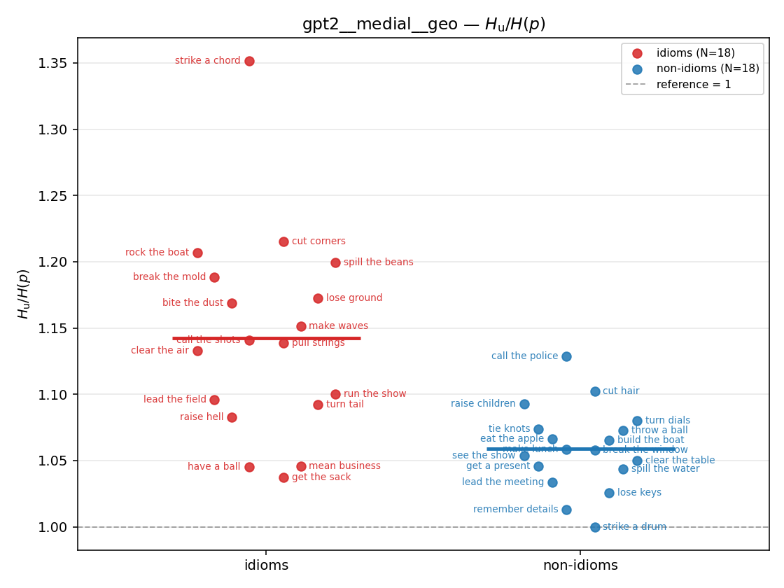 | 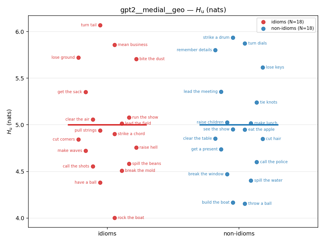 | 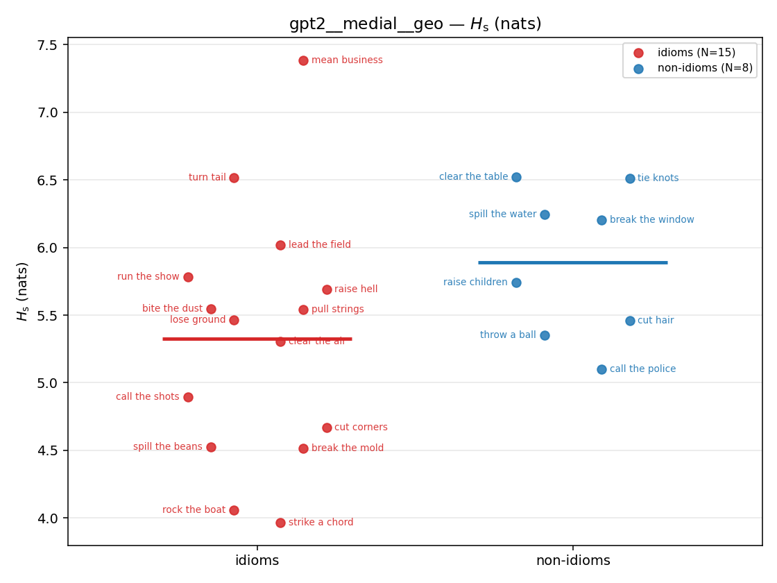 | 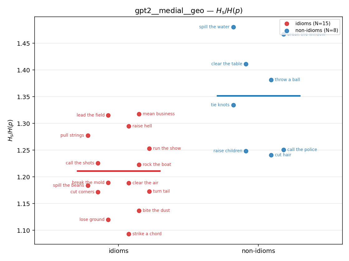 | 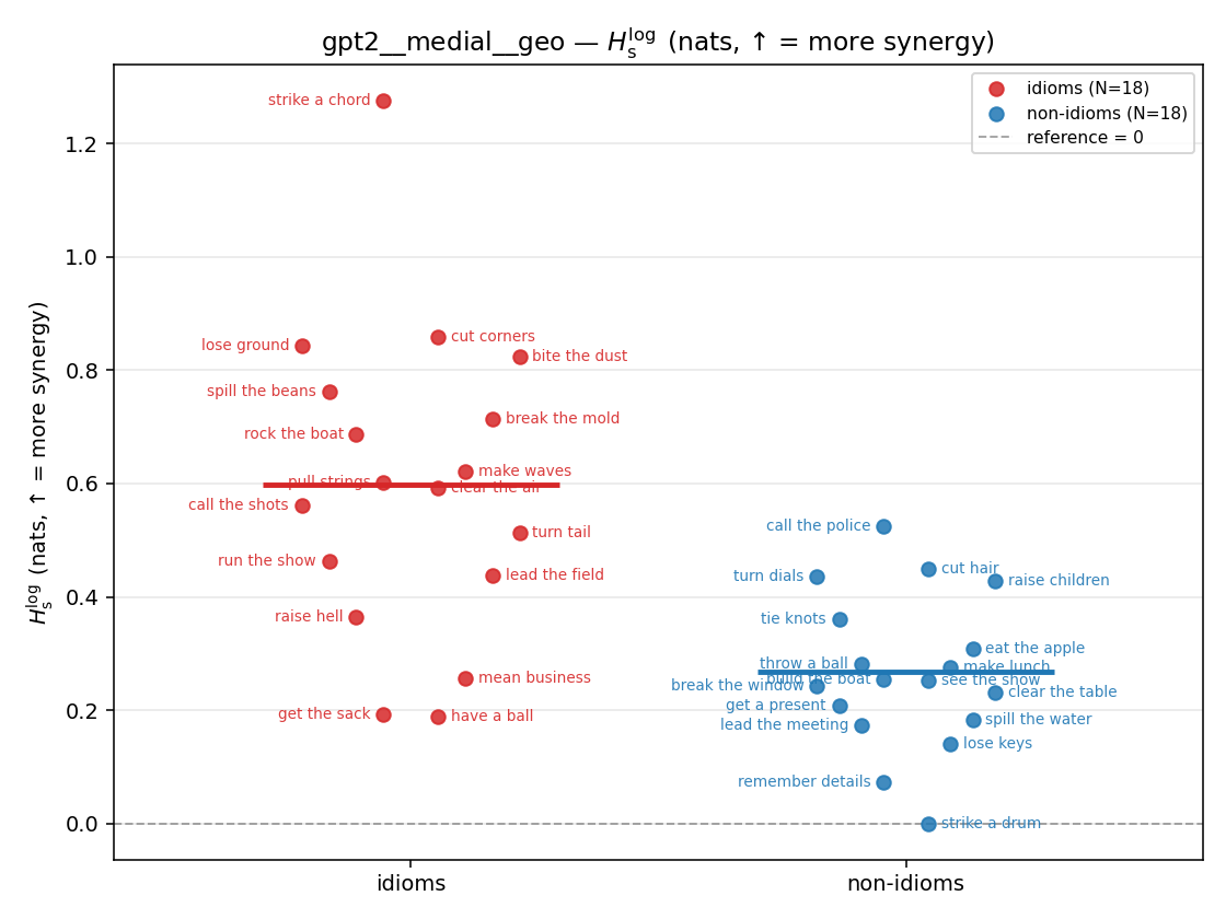 | 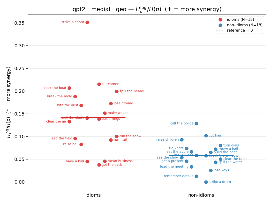 | 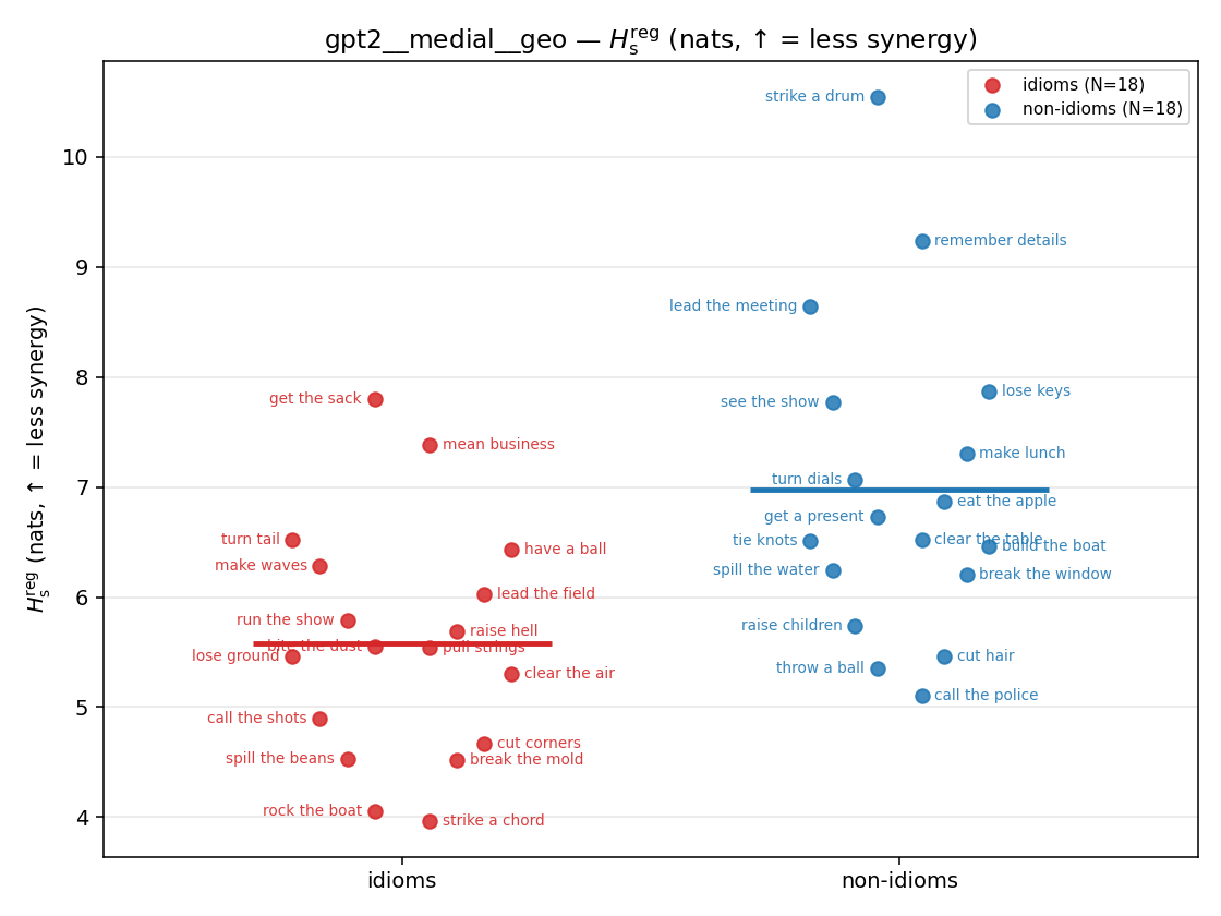 | 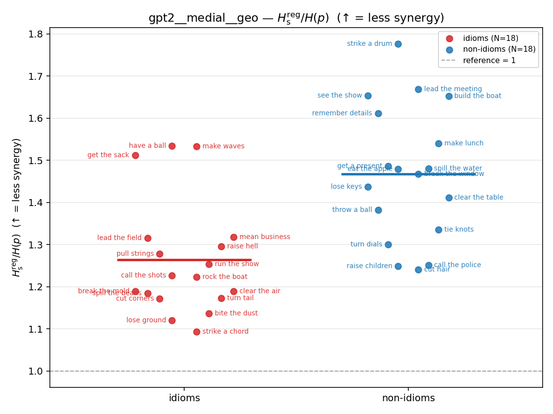 | 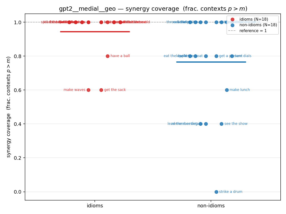 |
| mean ± 95% CI | 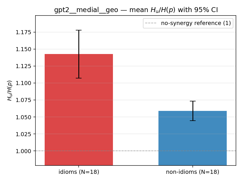 | 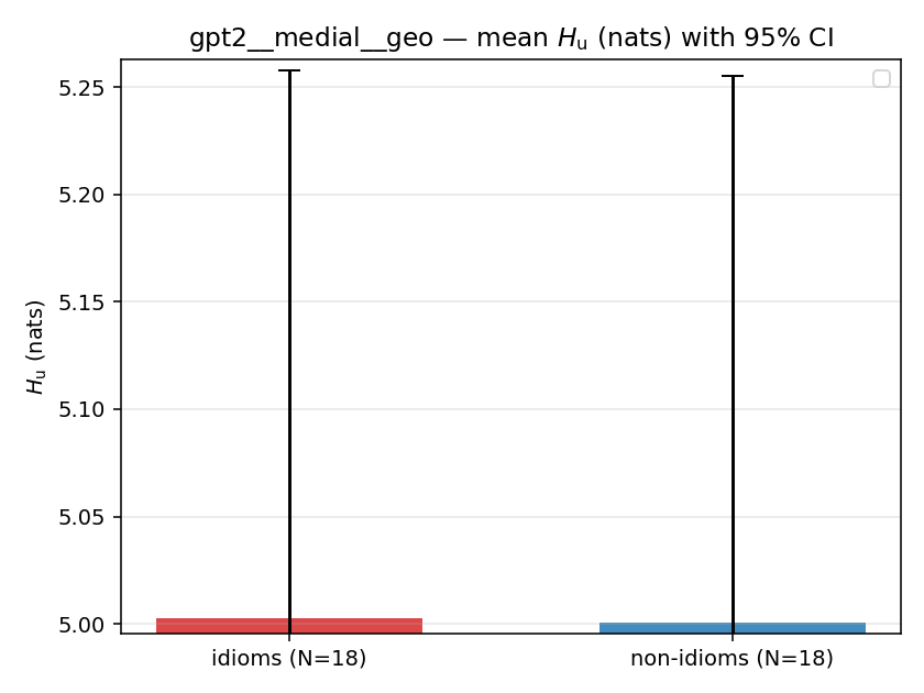 | 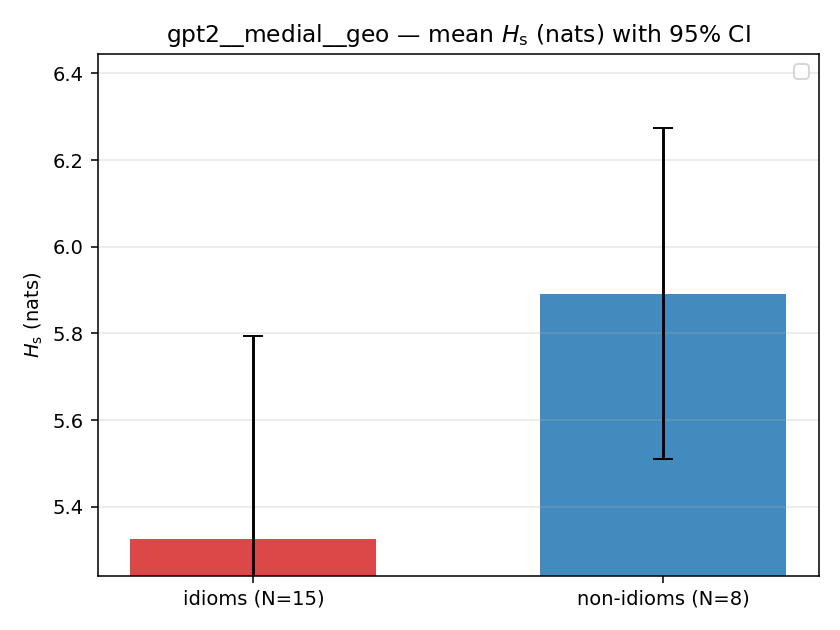 | 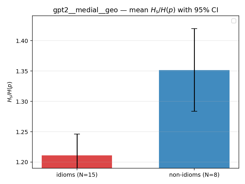 | 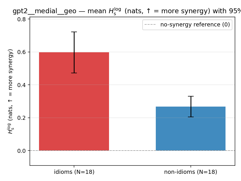 | 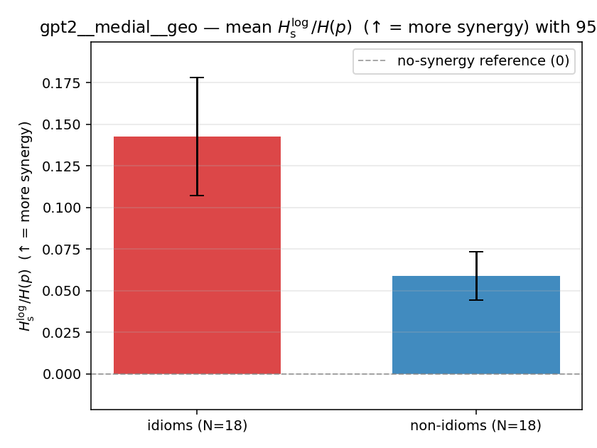 | 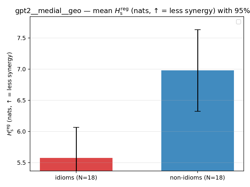 | 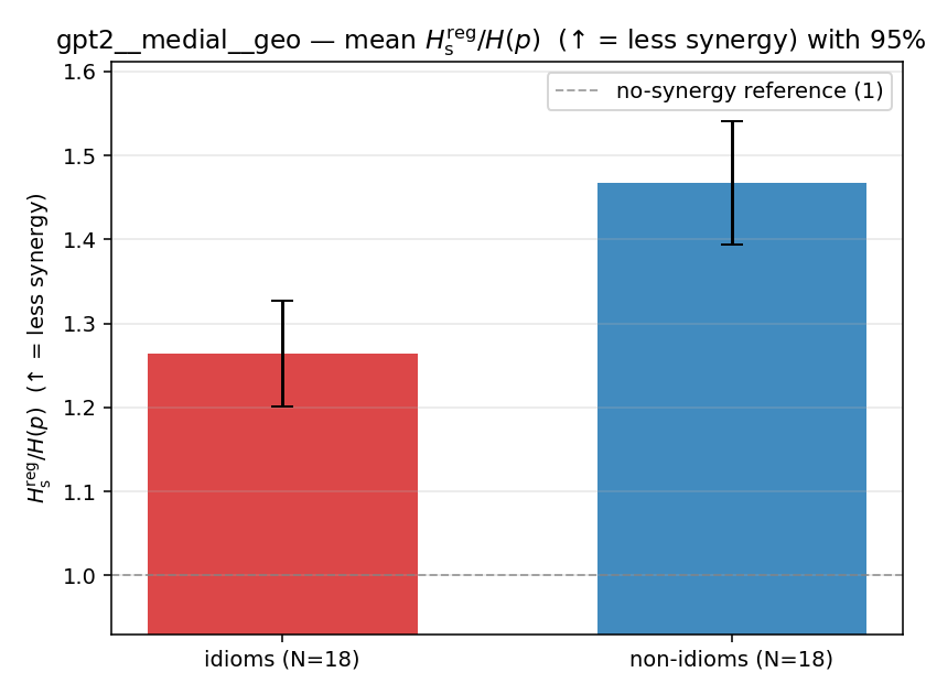 | 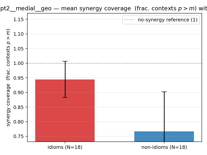 |
| per-idiom (sorted) | 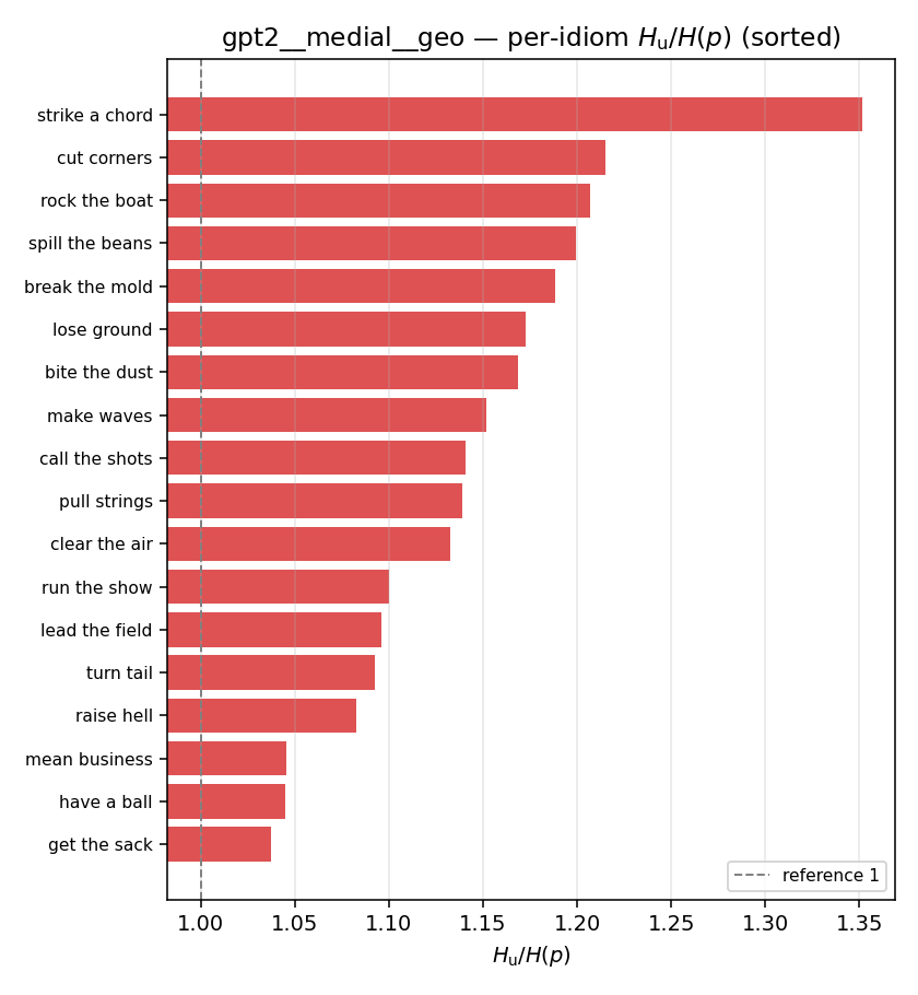 | 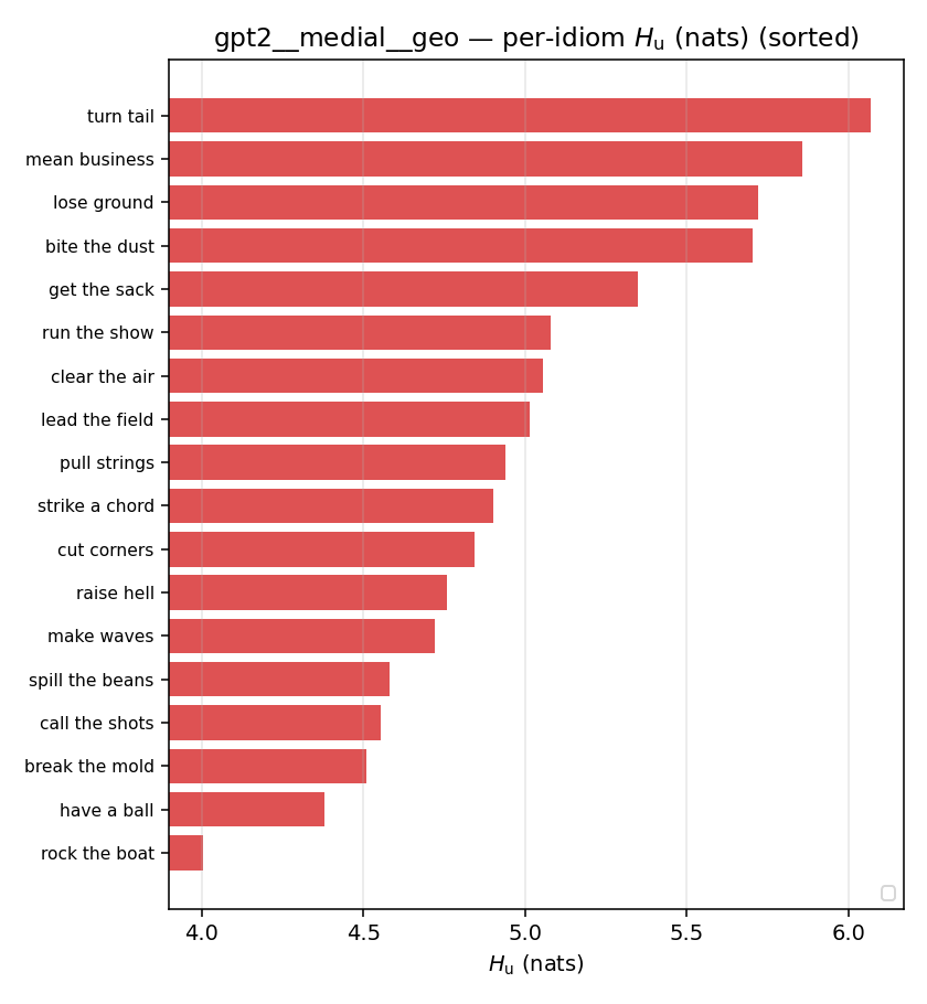 | 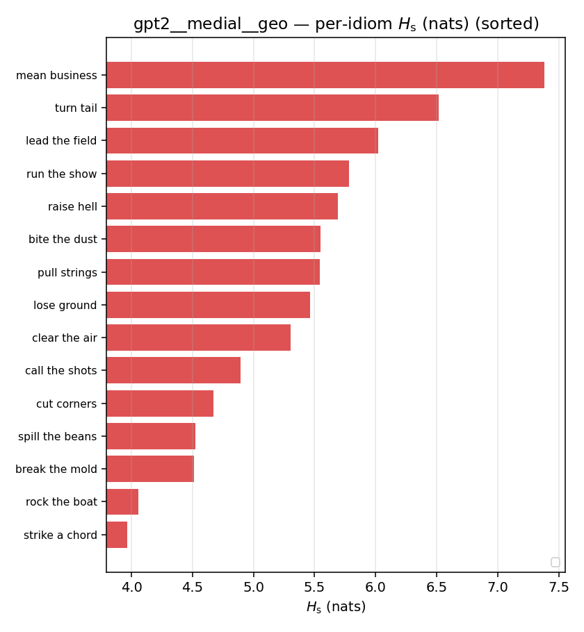 | 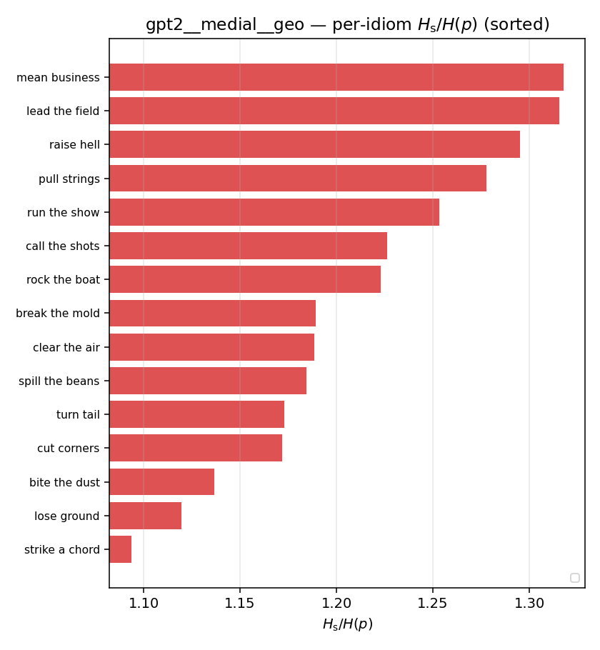 | 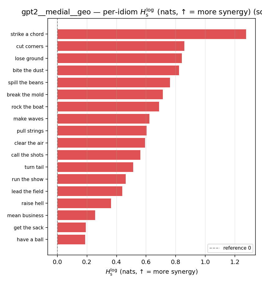 | 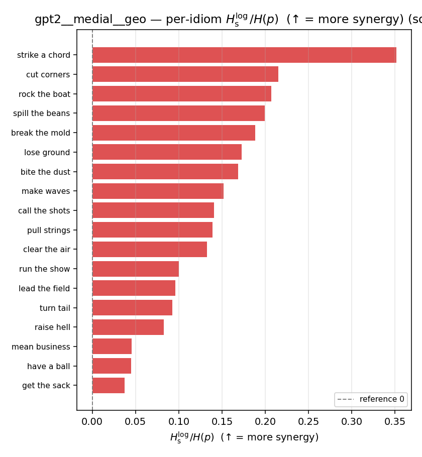 | 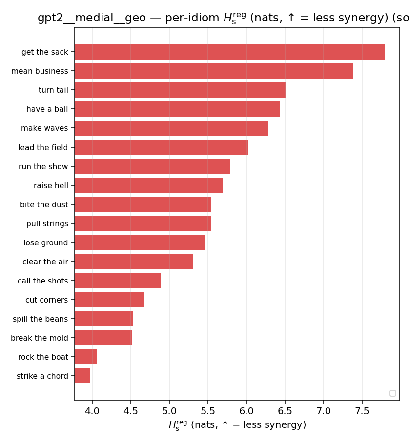 | 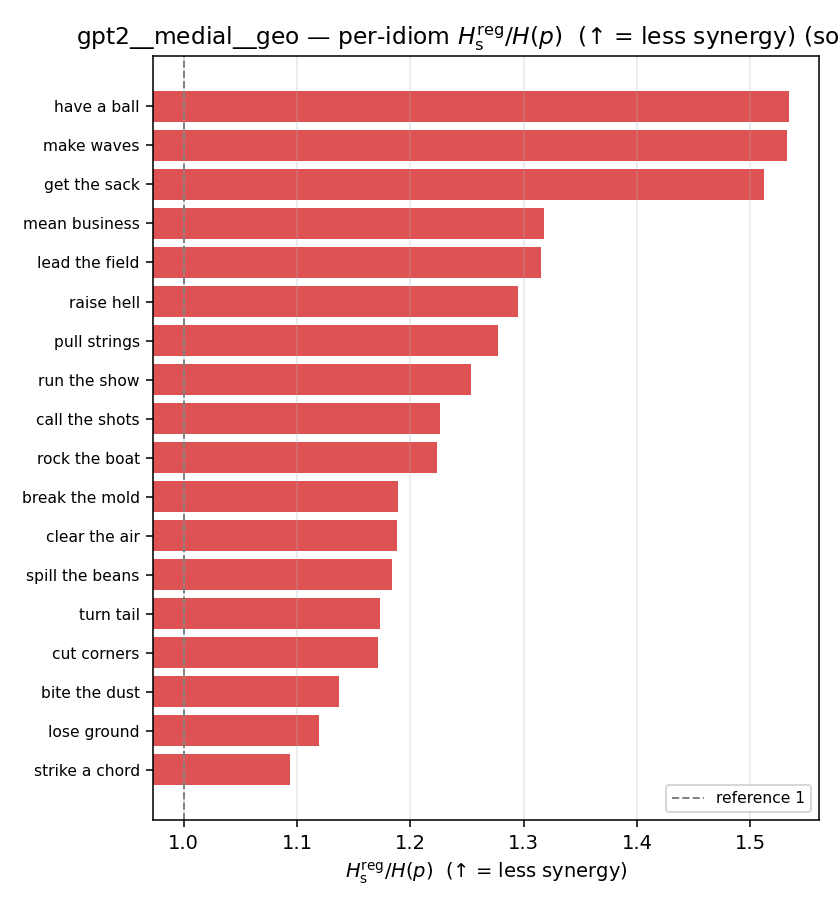 | 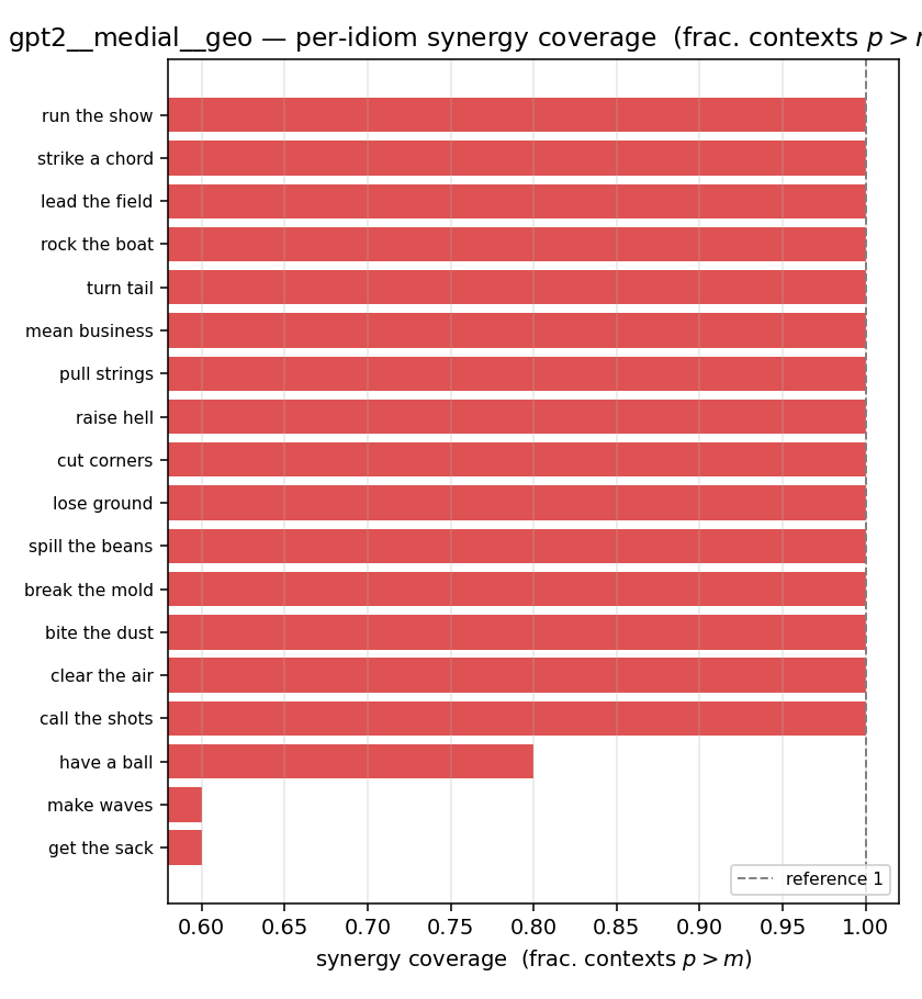 |
gpt2 · medial · joint gpt2__medial__joint
| Ĥu/Ĥ ↑syn | Ĥu | Ĥs ↓syn | Ĥs/Ĥ ↓syn | Ĥslog ↑syn | Ĥslog/Ĥ ↑syn | Ĥsreg ↓syn | Ĥsreg/Ĥ ↓syn | f̂syn ↑syn | |
|---|---|---|---|---|---|---|---|---|---|
| strip (per-phrase) | 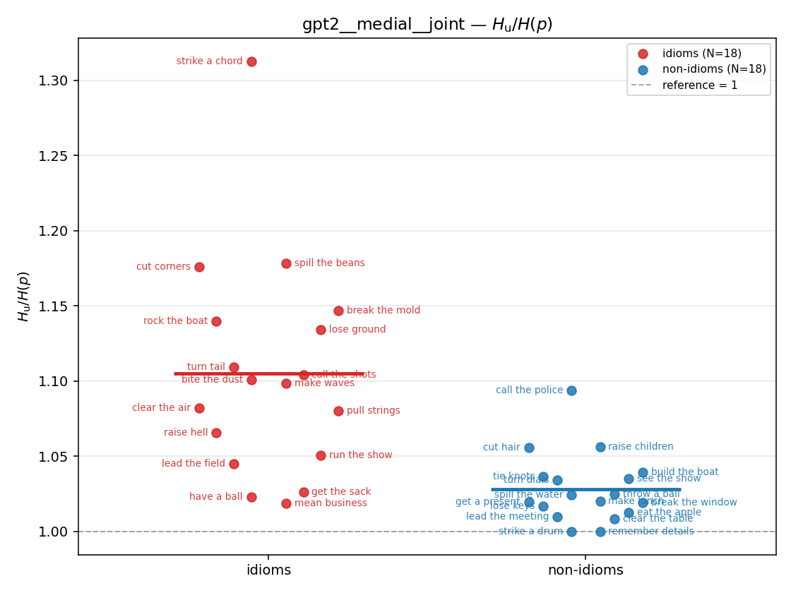 | 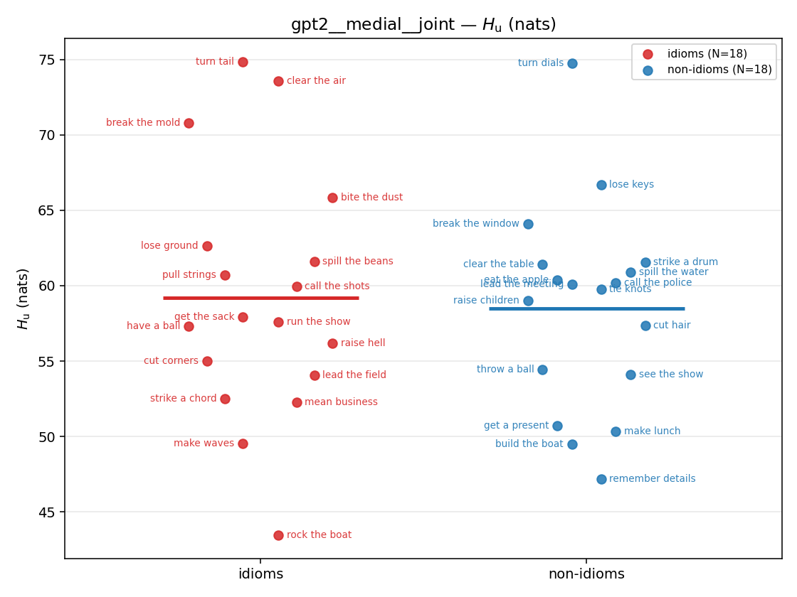 | 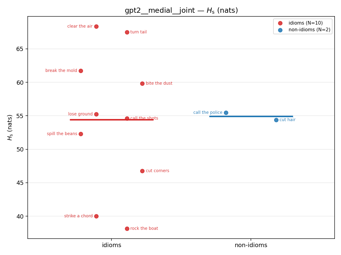 | 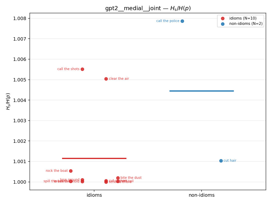 | 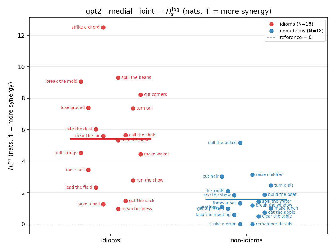 | 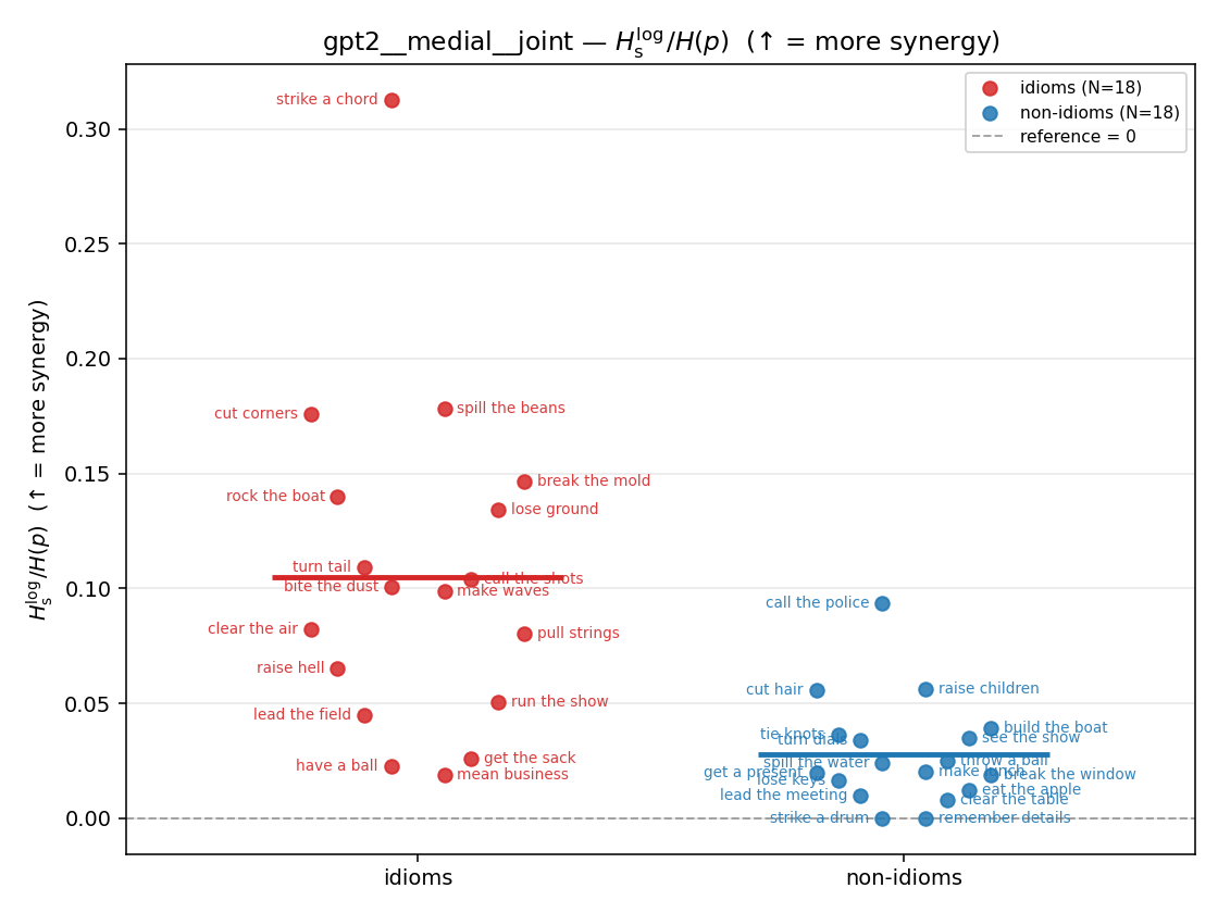 | 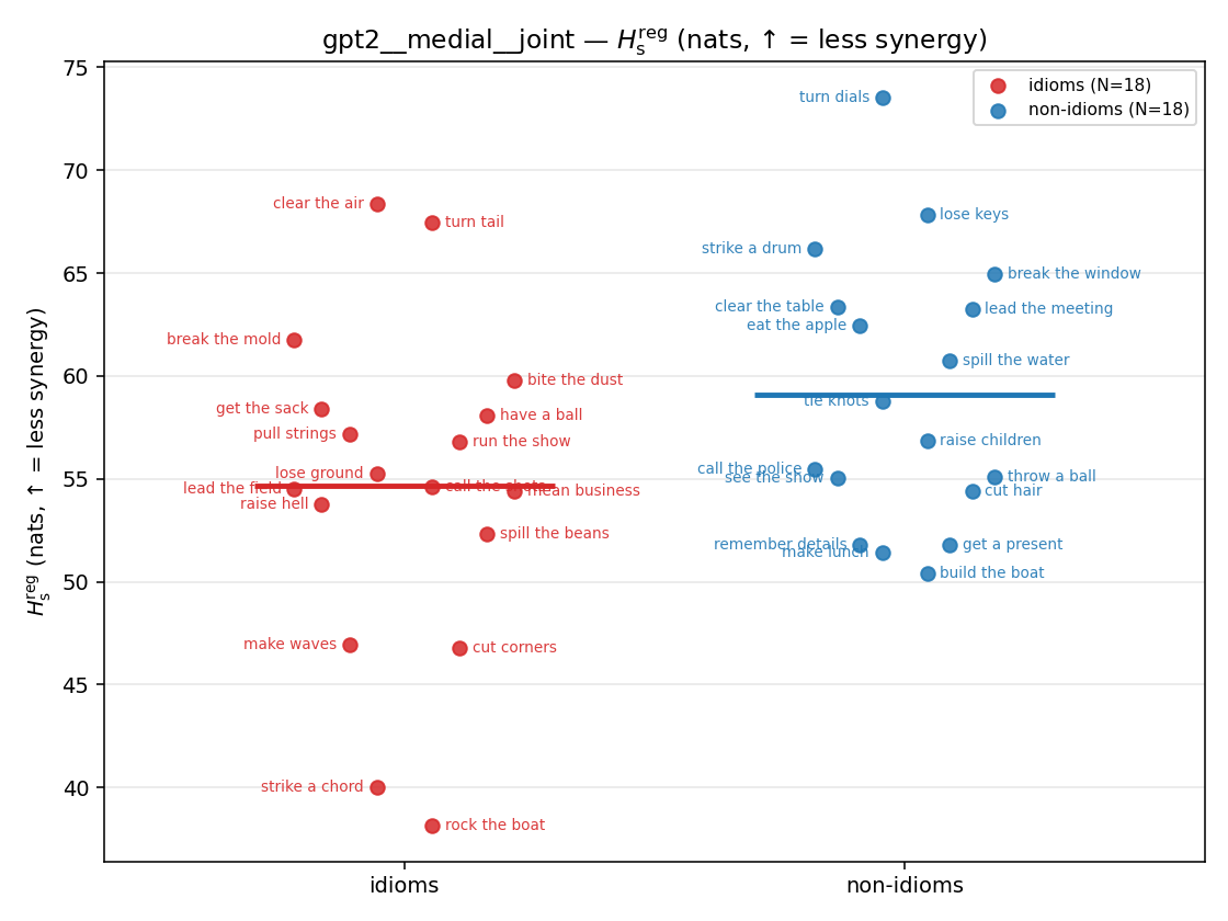 | 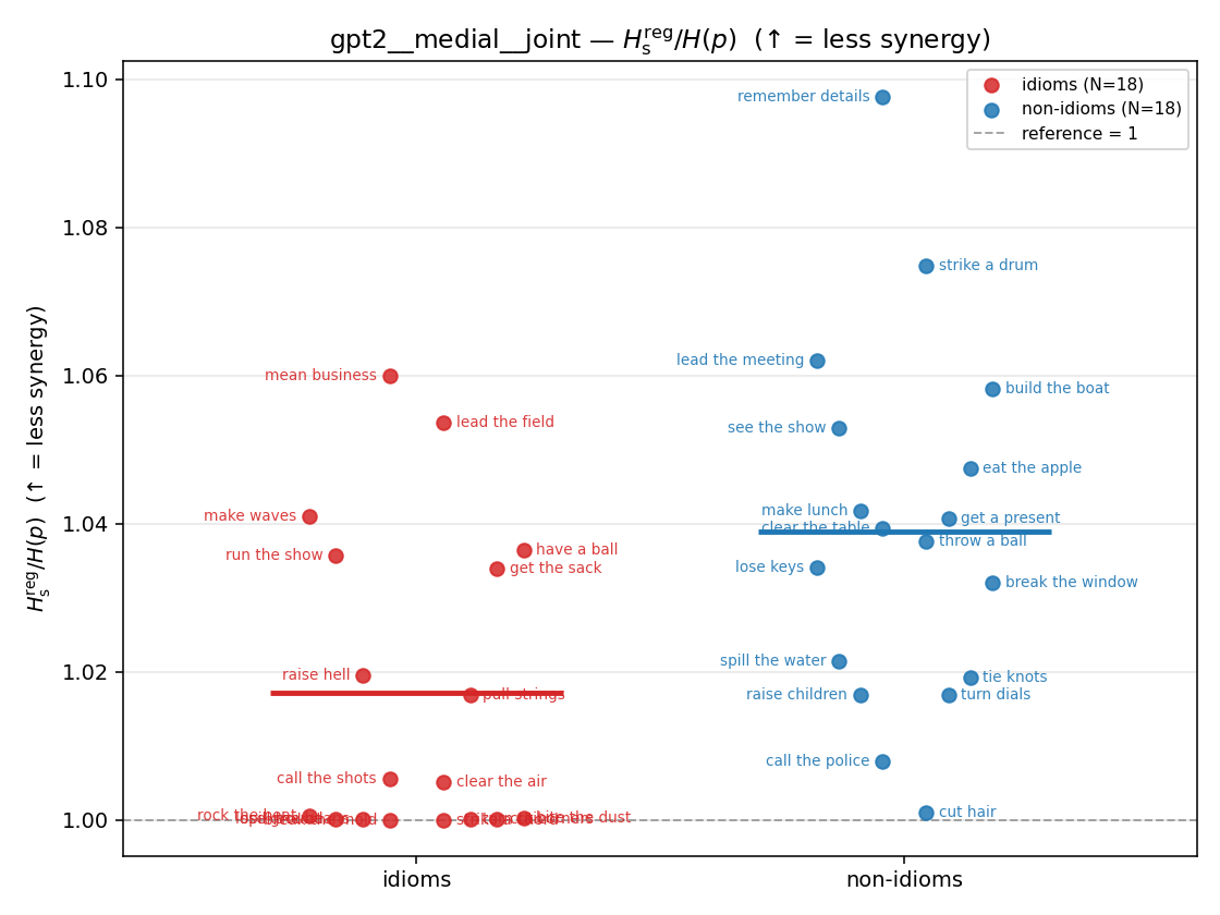 | 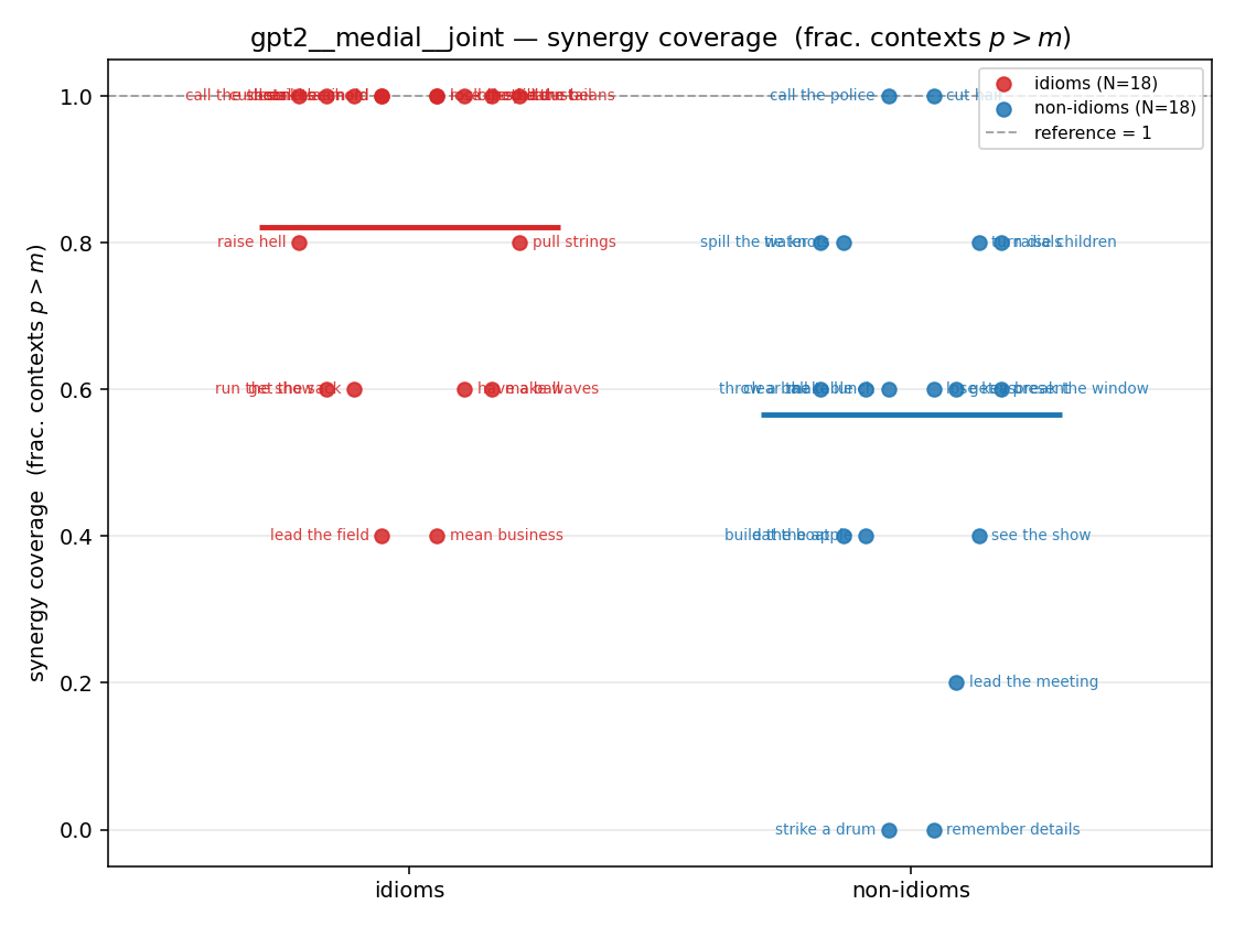 |
| mean ± 95% CI | 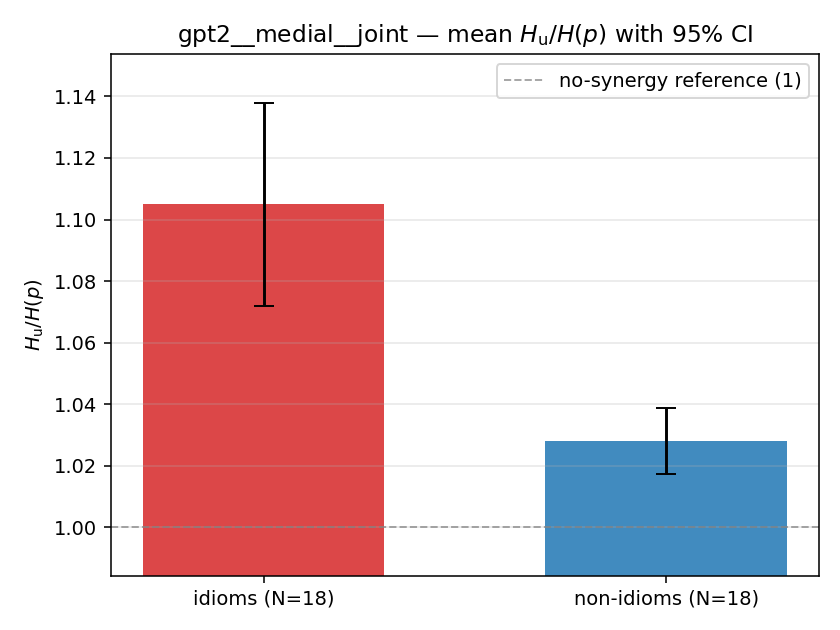 | 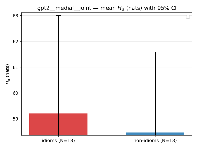 | 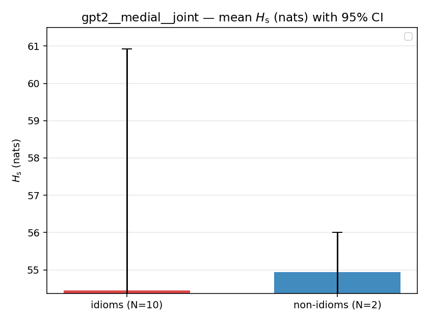 | 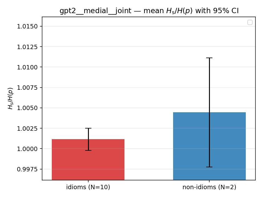 | 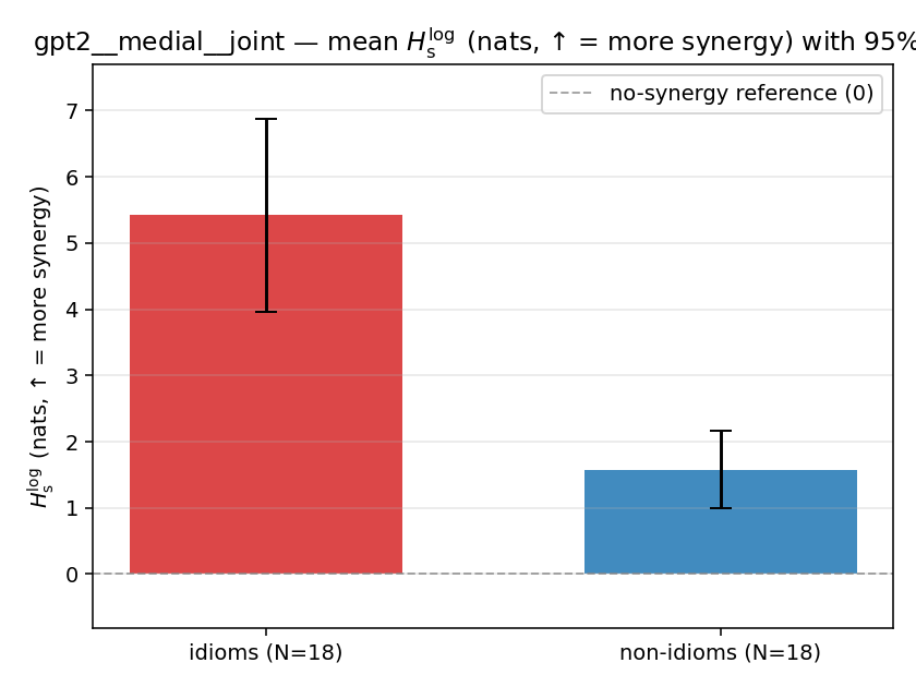 | 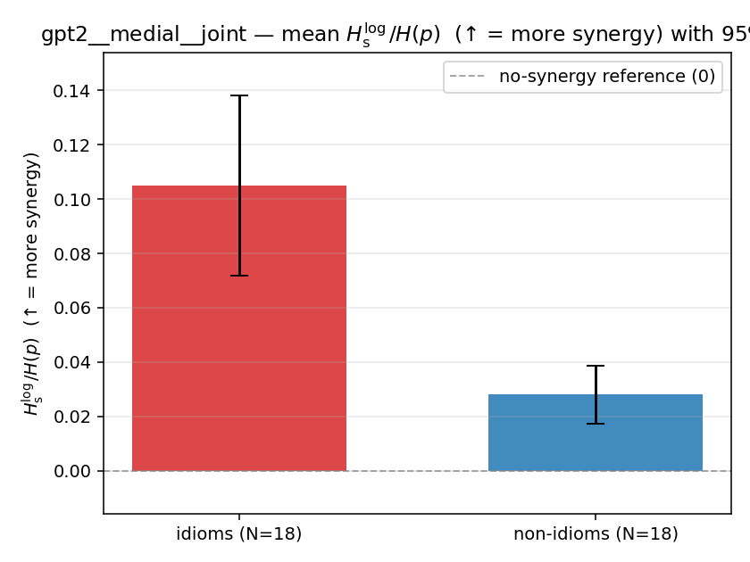 | 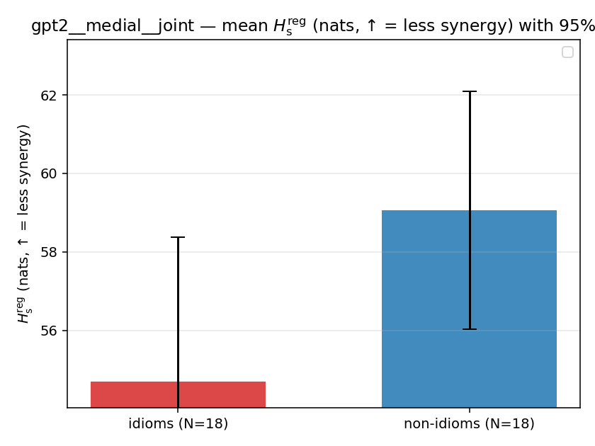 | 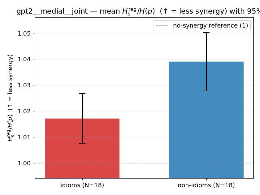 | 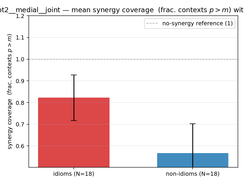 |
| per-idiom (sorted) | 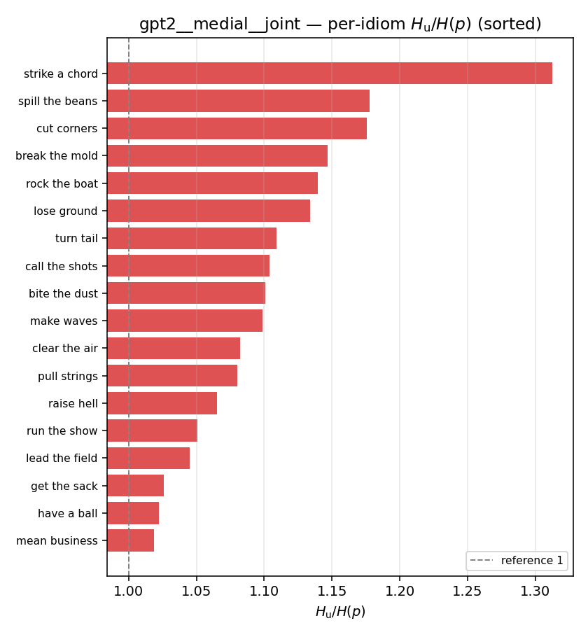 | 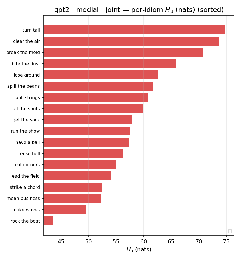 | 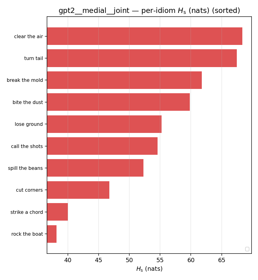 | 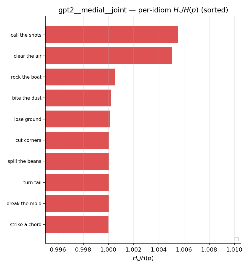 | 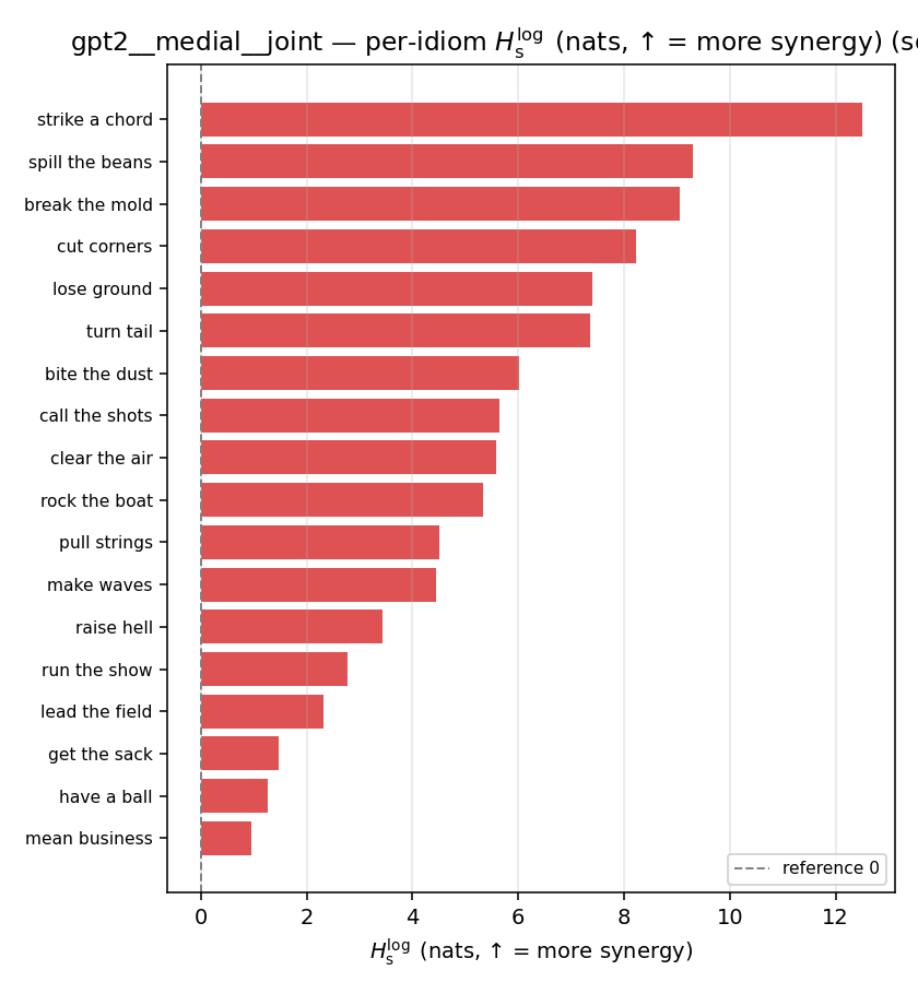 | 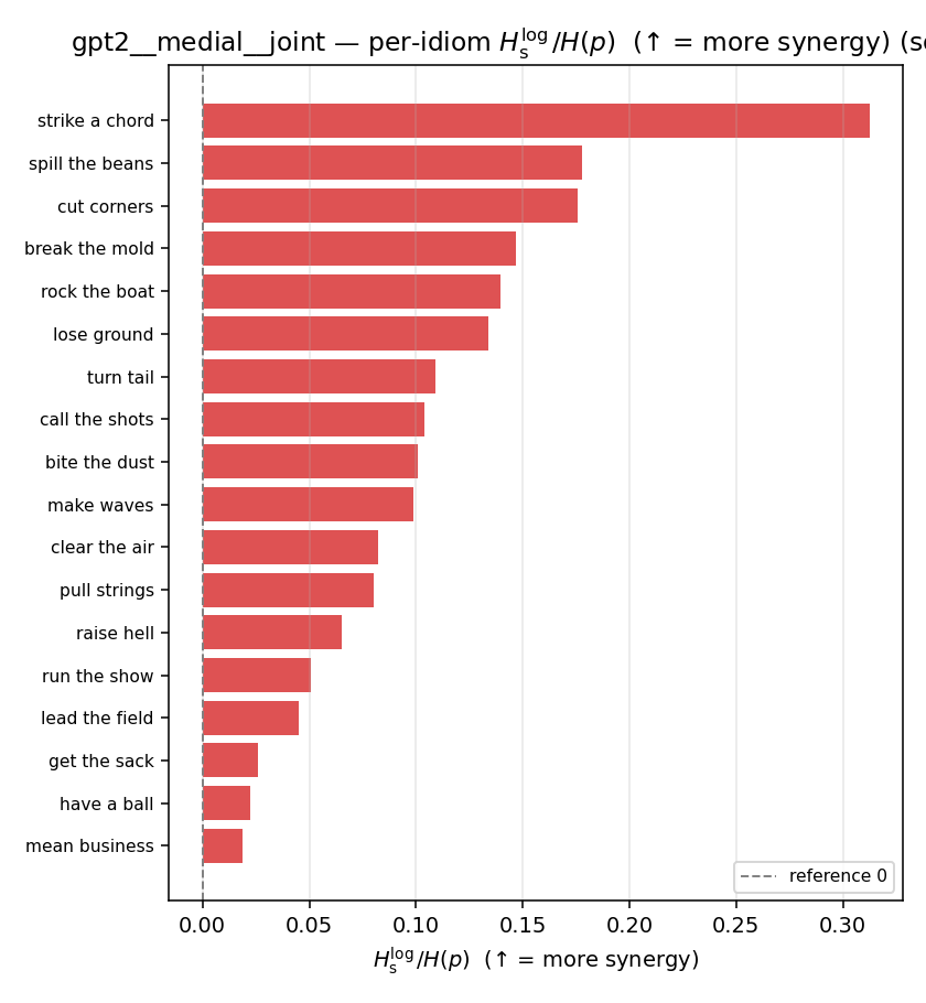 | 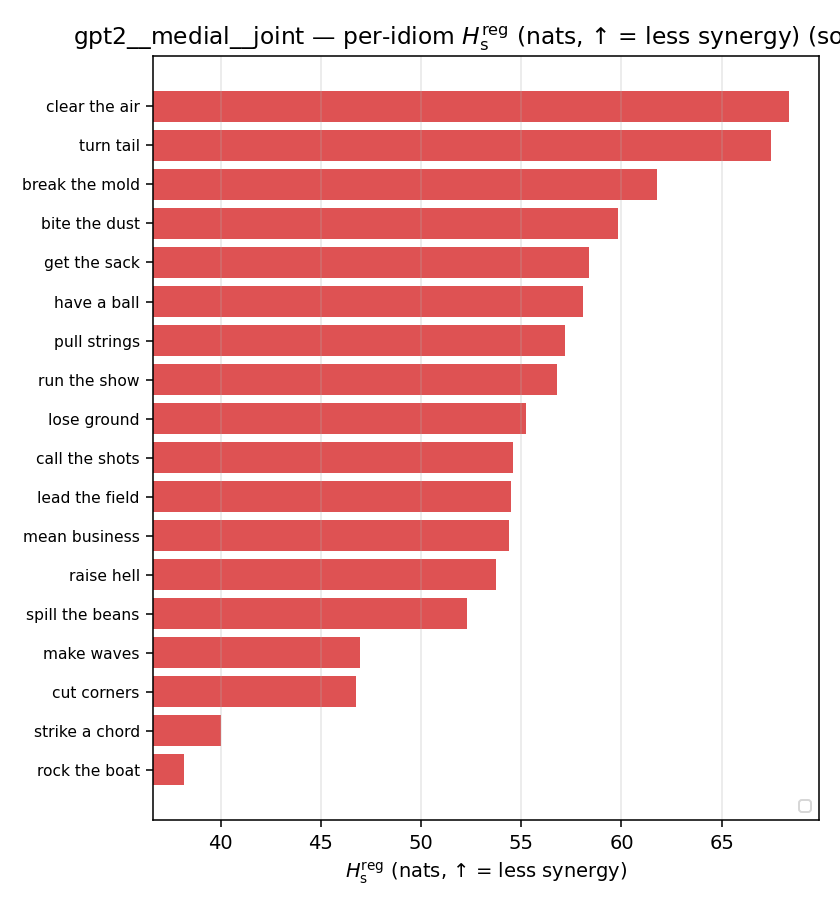 | 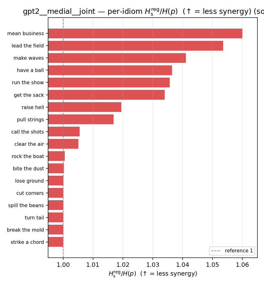 | 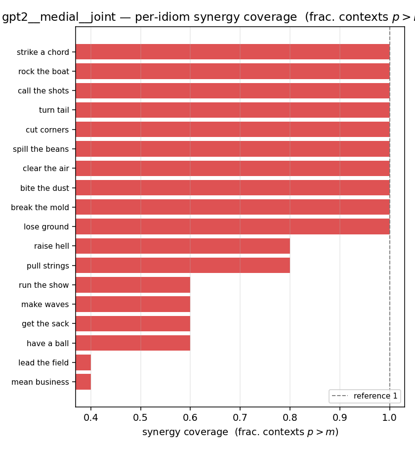 |
gpt2 · full · geo gpt2__full__geo
| Ĥu/Ĥ ↑syn | Ĥu | Ĥs ↓syn | Ĥs/Ĥ ↓syn | Ĥslog ↑syn | Ĥslog/Ĥ ↑syn | Ĥsreg ↓syn | Ĥsreg/Ĥ ↓syn | f̂syn ↑syn | |
|---|---|---|---|---|---|---|---|---|---|
| strip (per-phrase) | 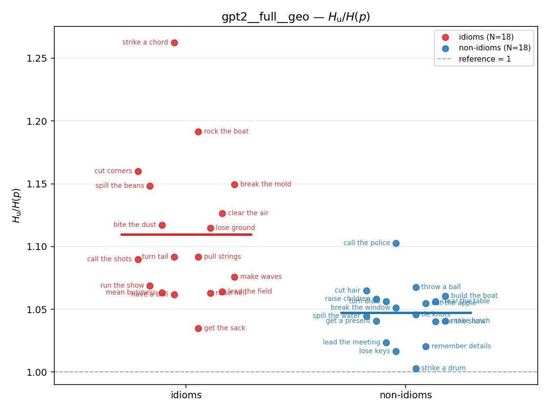 | 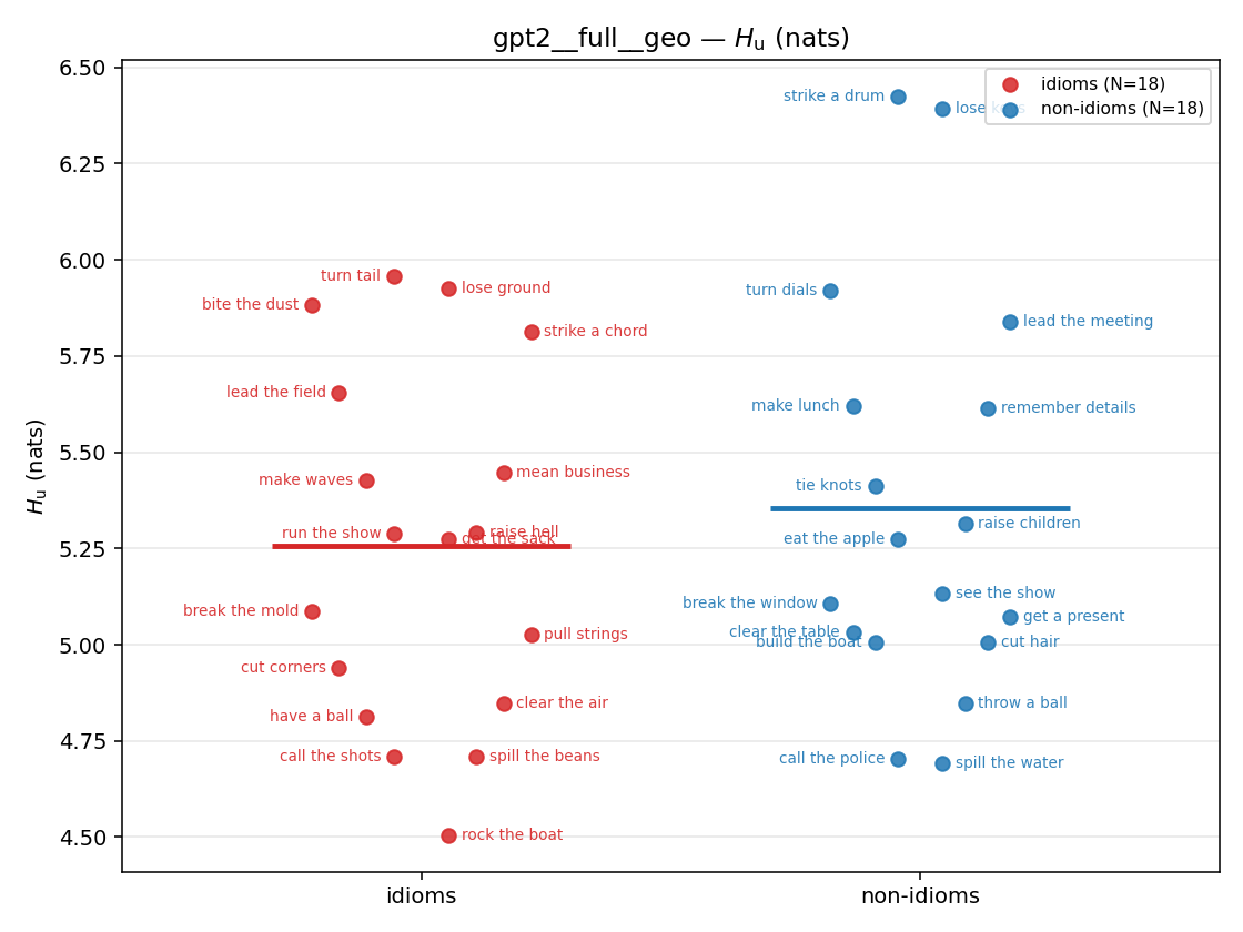 | 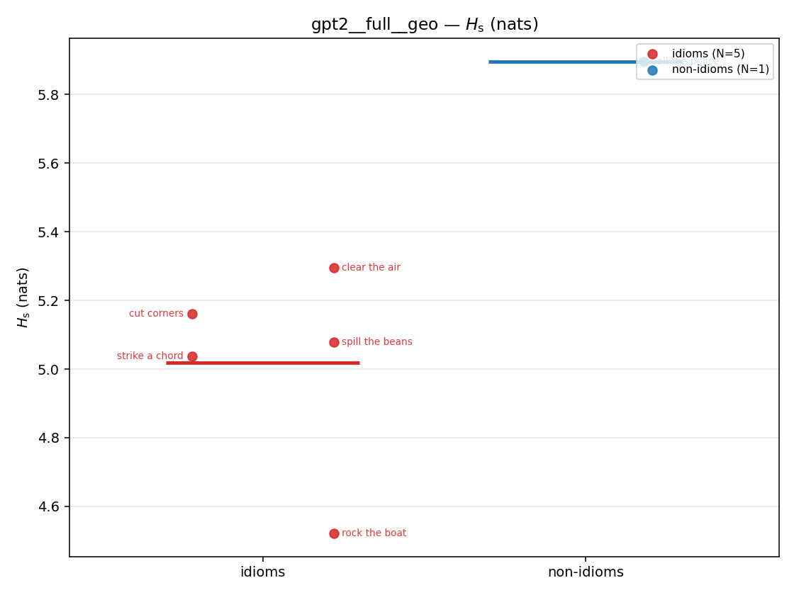 | 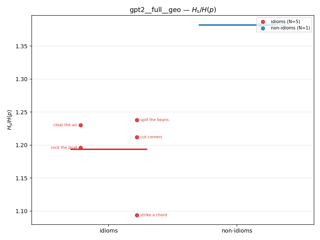 | 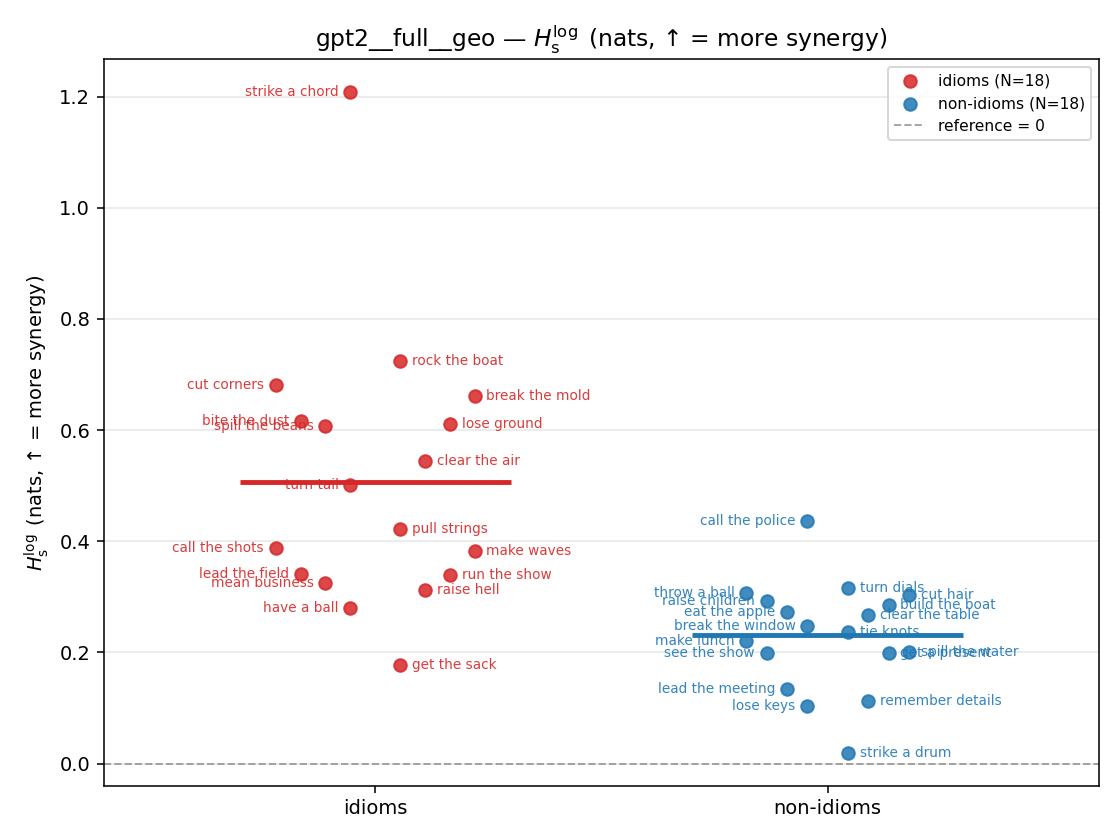 | 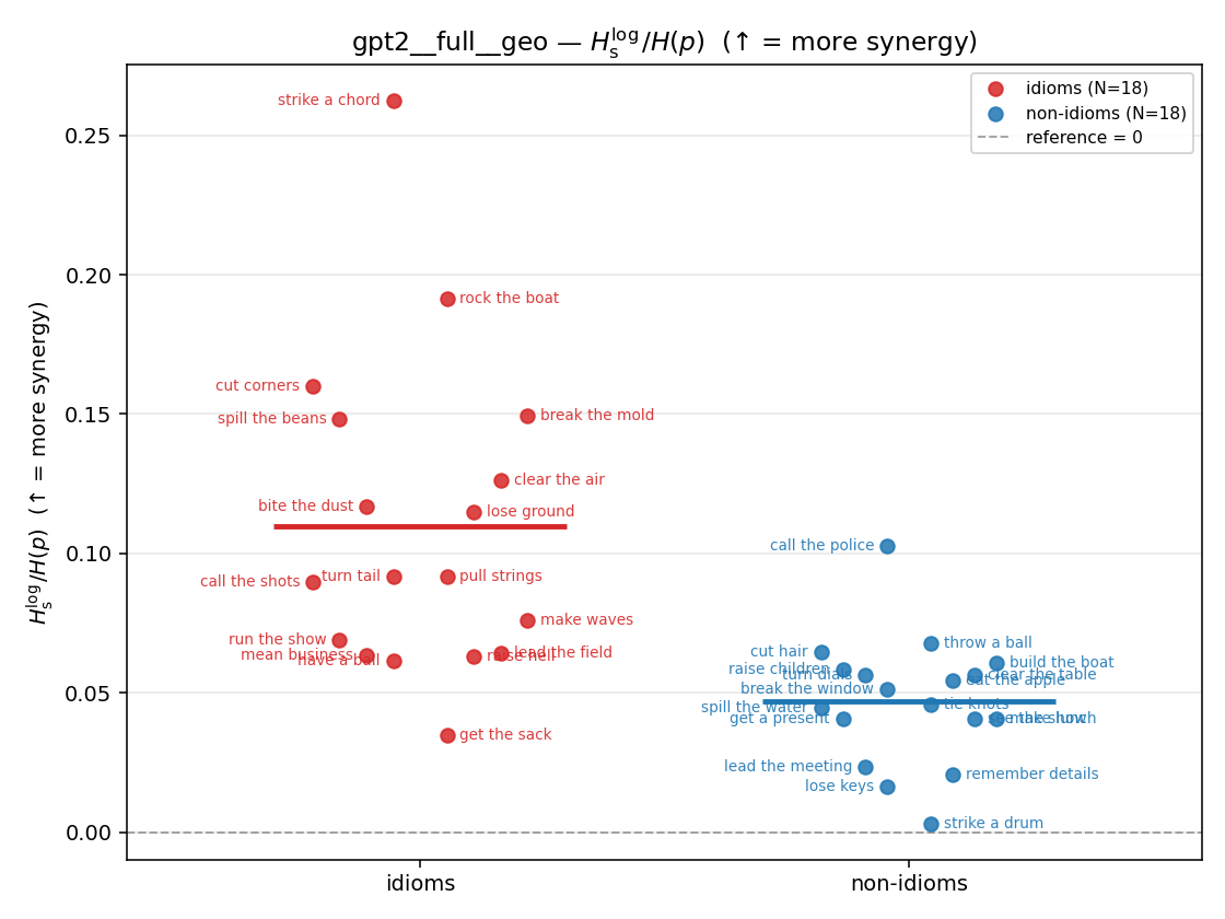 | 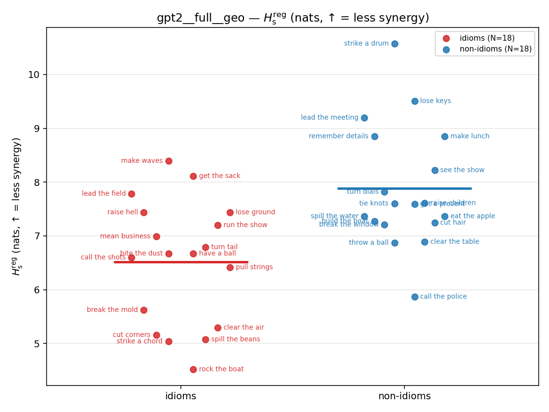 | 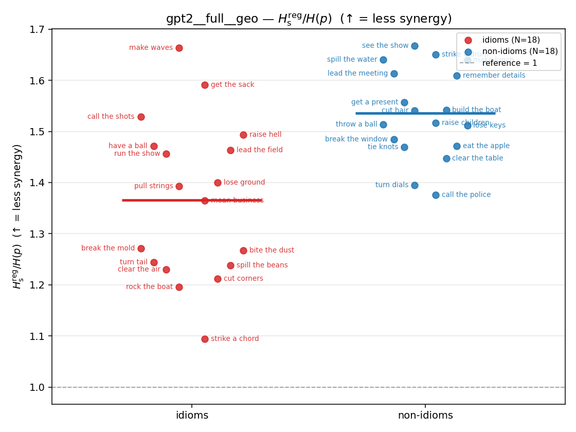 | 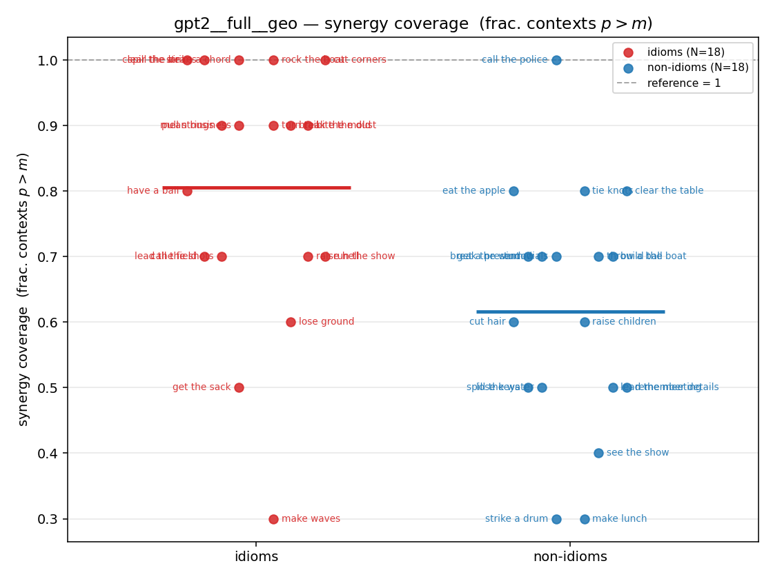 |
| mean ± 95% CI | 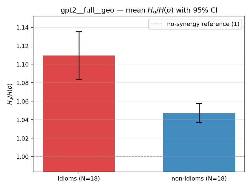 | 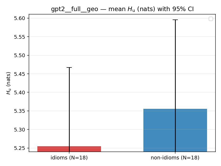 | 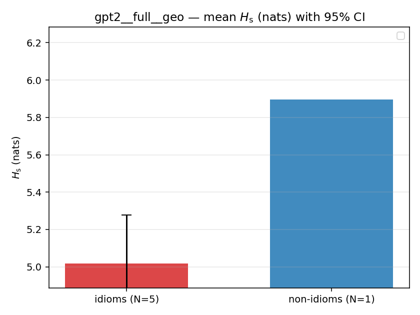 | 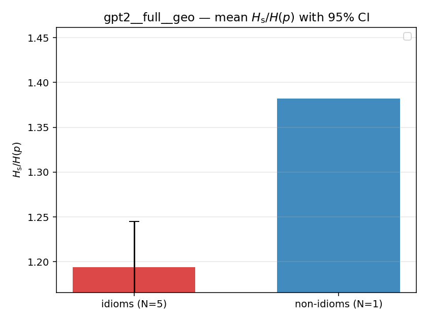 | 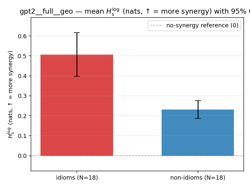 | 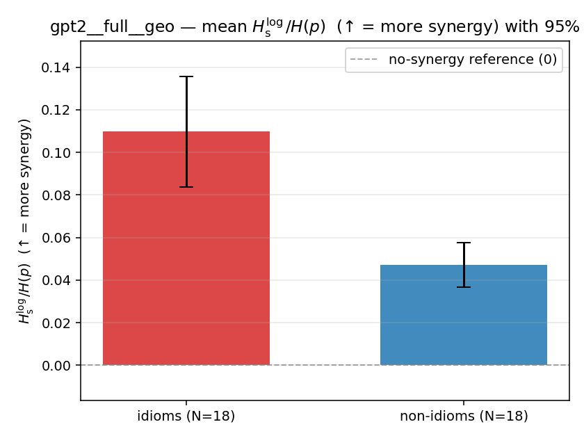 | 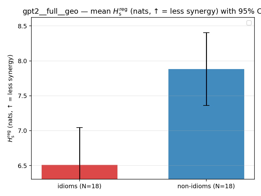 | 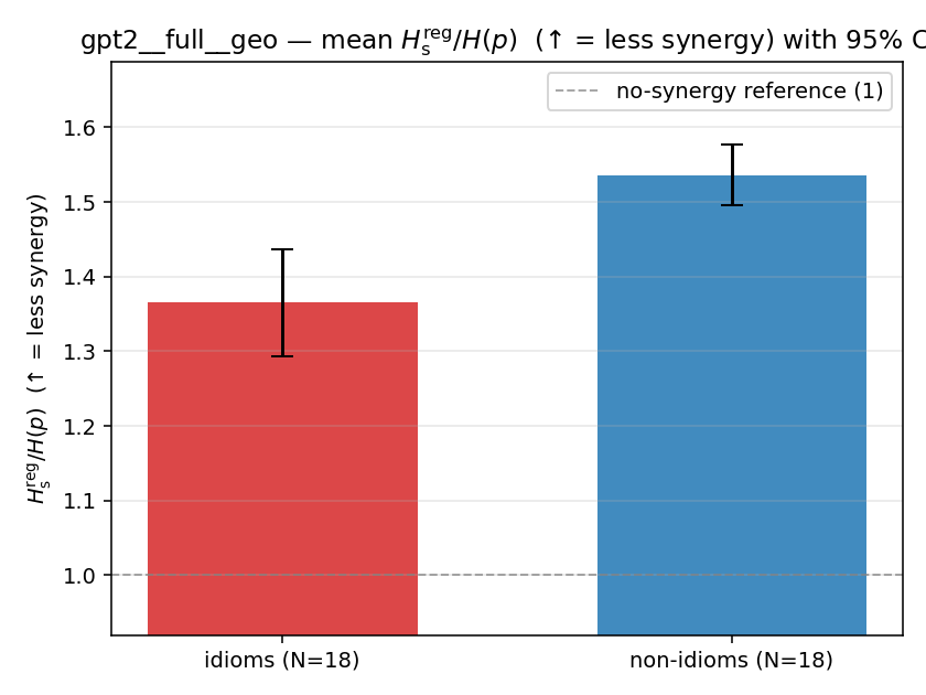 | 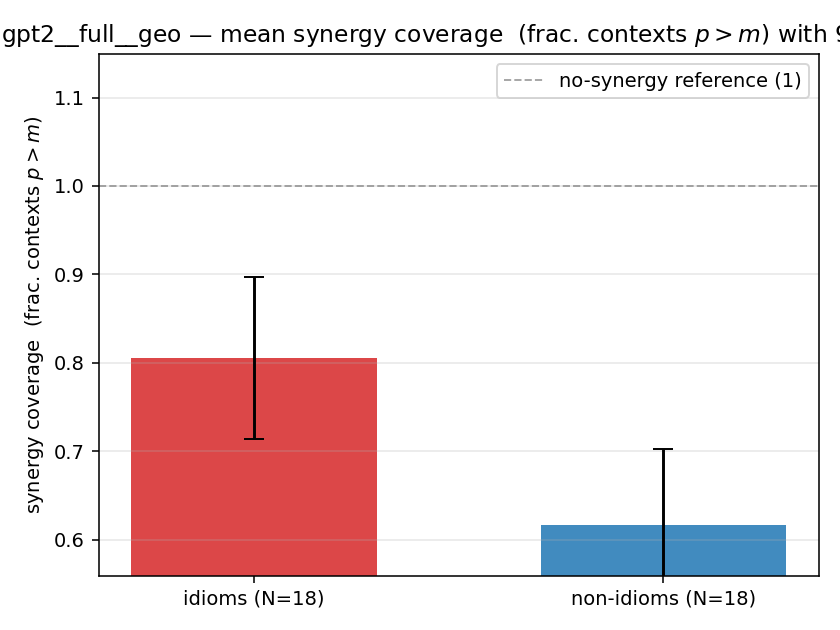 |
| per-idiom (sorted) | 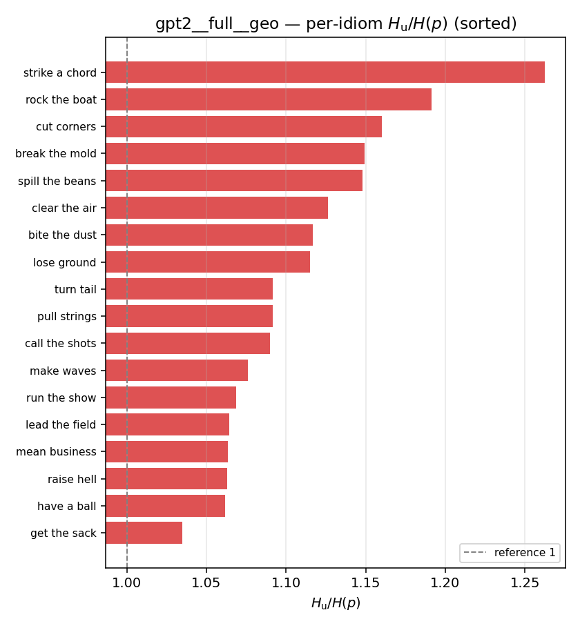 | 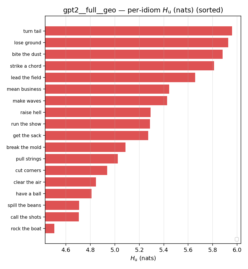 | 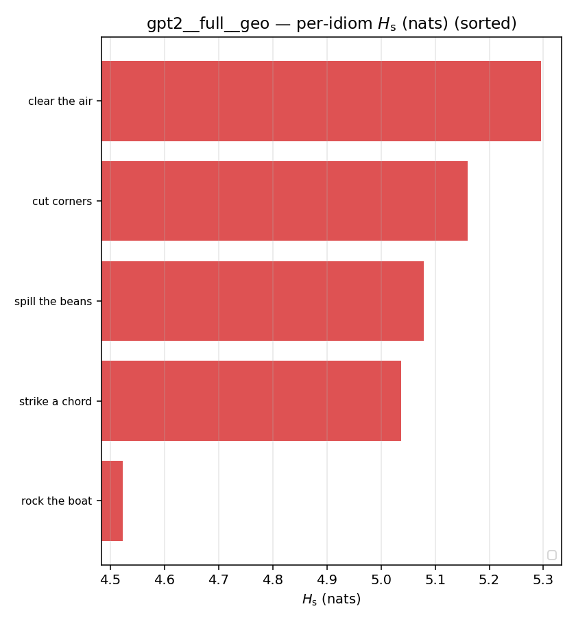 | 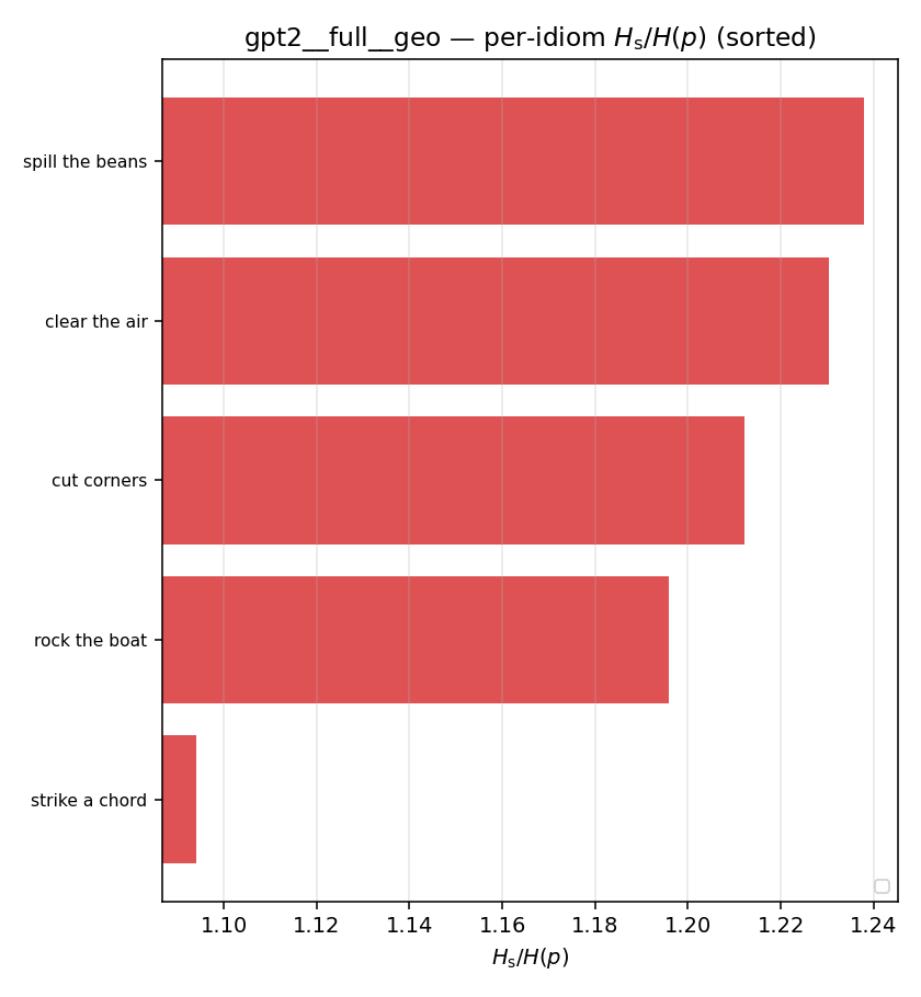 | 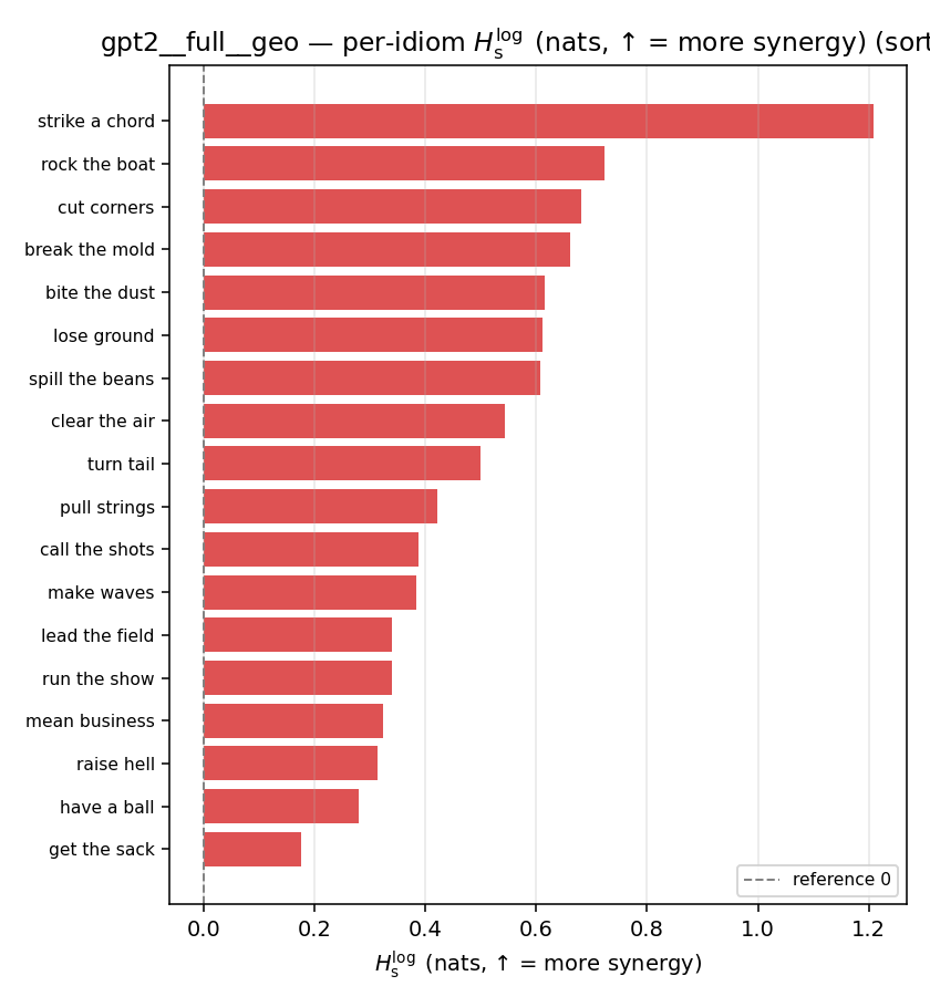 | 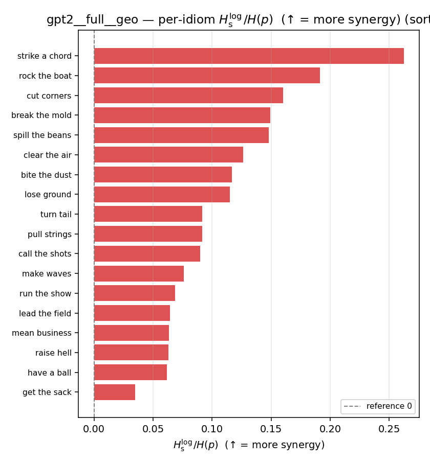 | 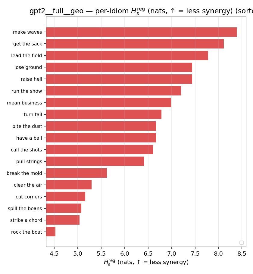 | 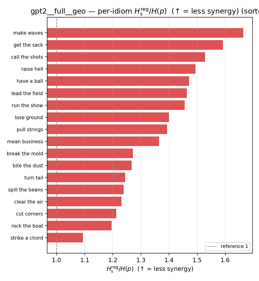 | 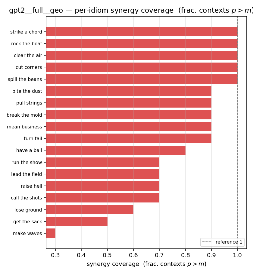 |
gpt2 · full · joint gpt2__full__joint
| Ĥu/Ĥ ↑syn | Ĥu | Ĥs ↓syn | Ĥs/Ĥ ↓syn | Ĥslog ↑syn | Ĥslog/Ĥ ↑syn | Ĥsreg ↓syn | Ĥsreg/Ĥ ↓syn | f̂syn ↑syn | |
|---|---|---|---|---|---|---|---|---|---|
| strip (per-phrase) | 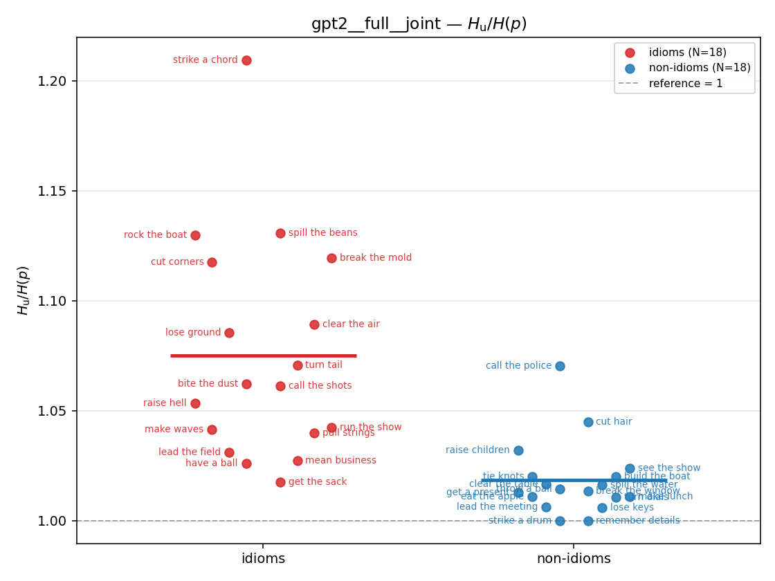 | 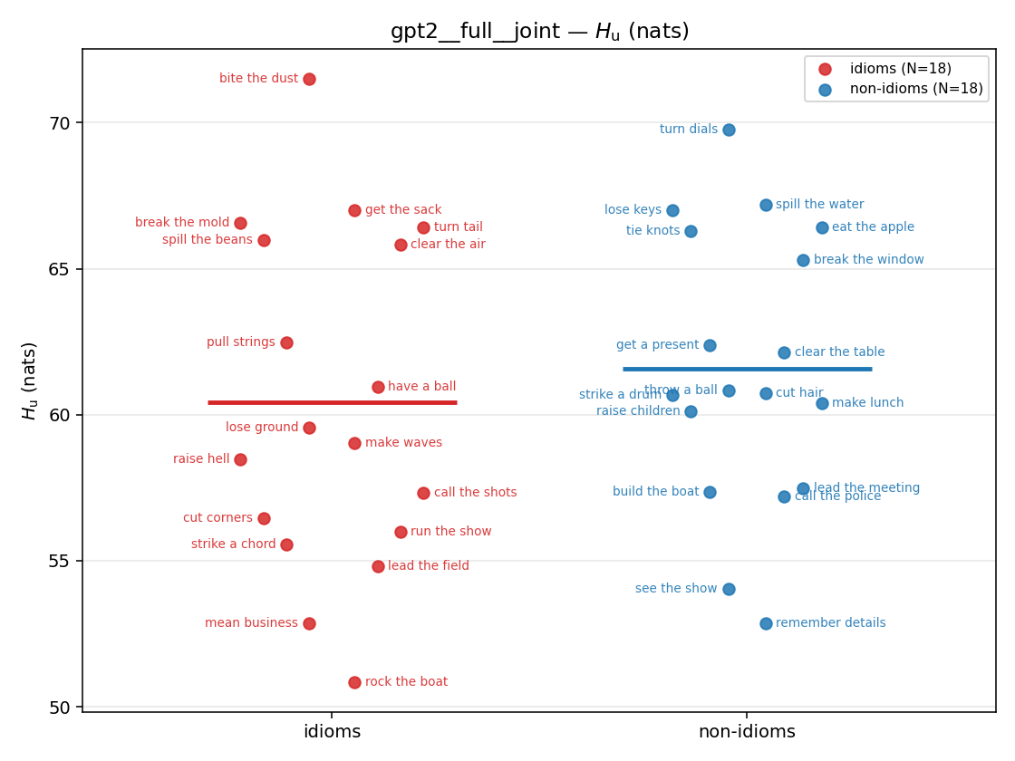 | 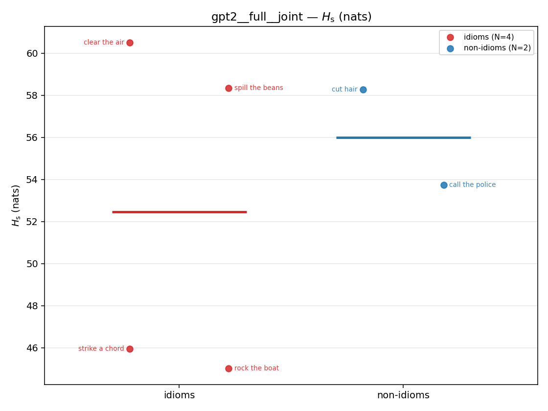 | 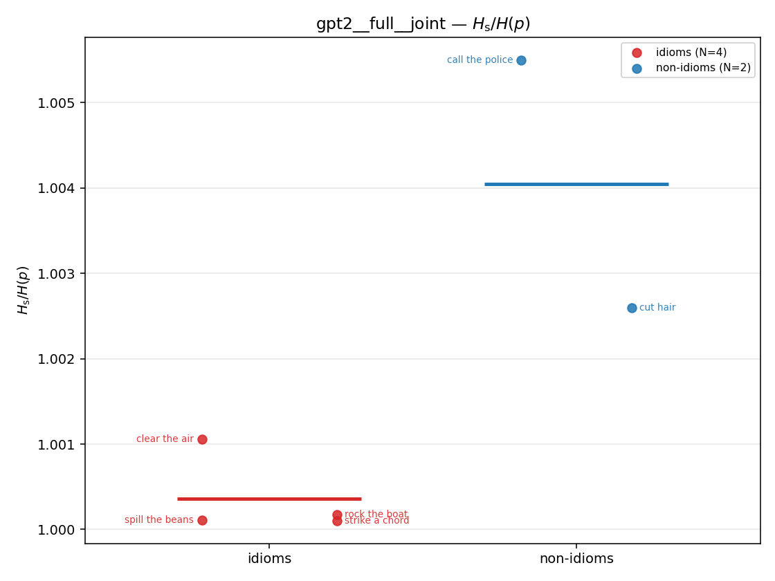 | 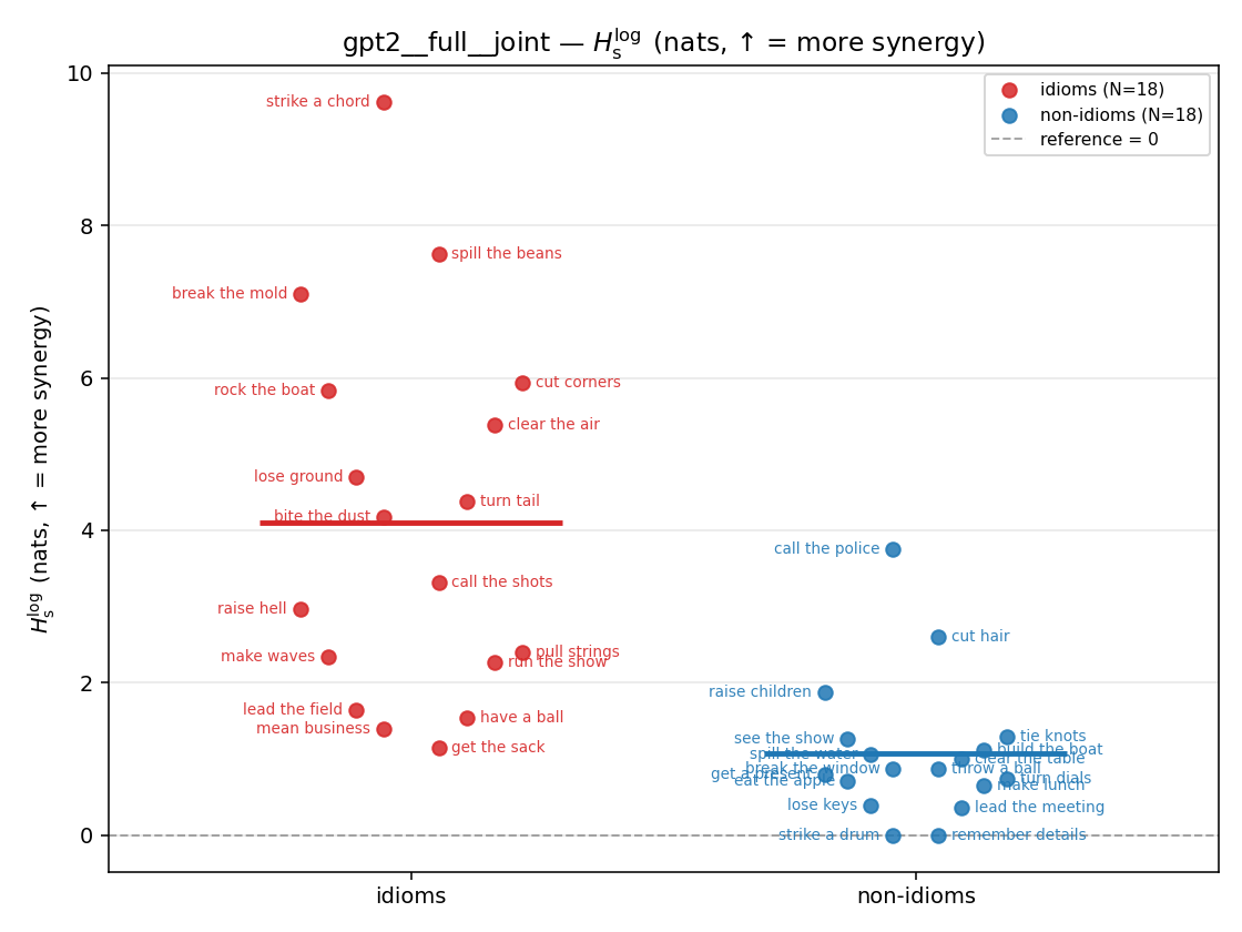 | 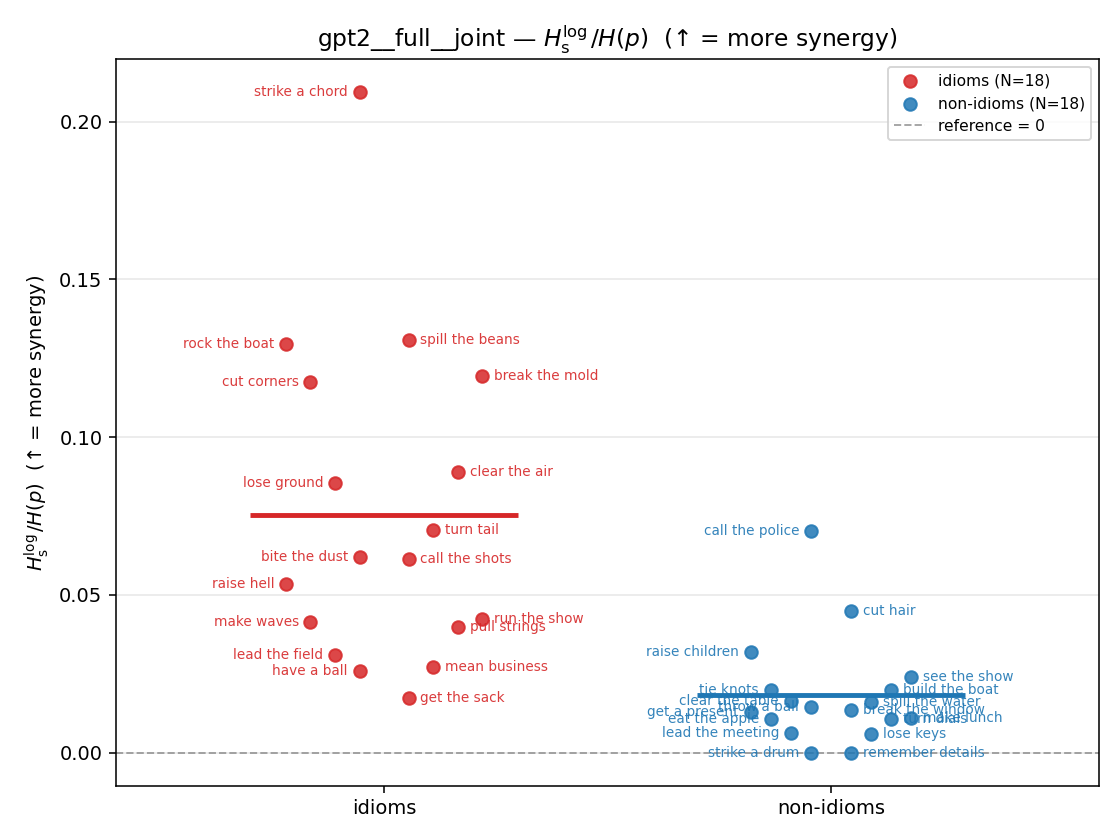 | 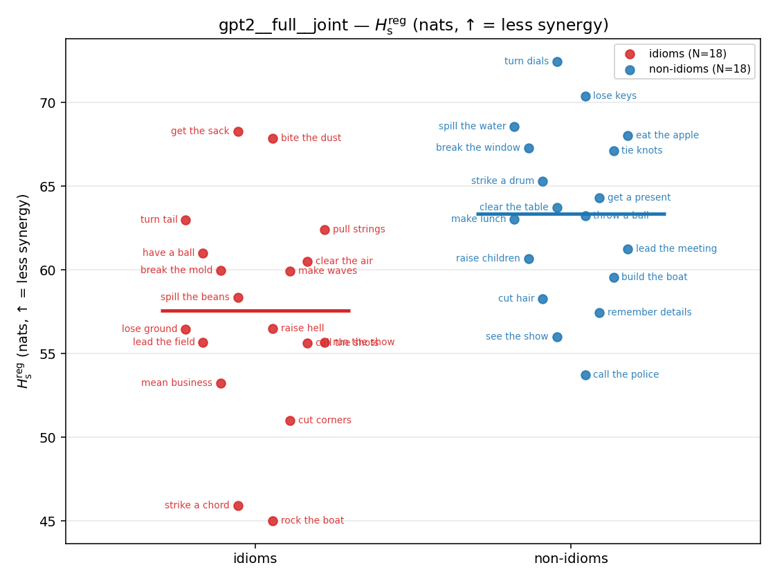 | 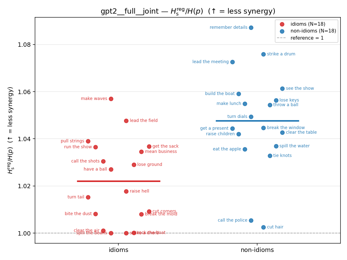 | 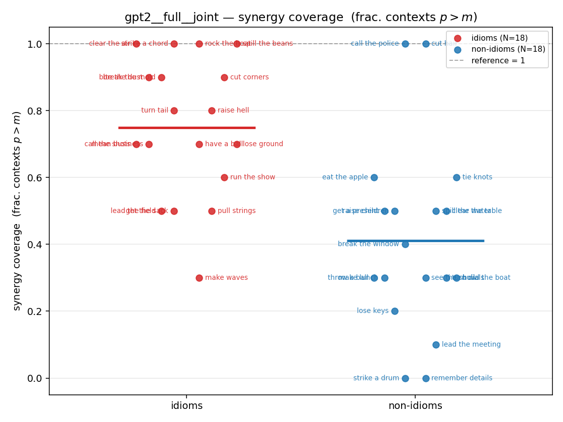 |
| mean ± 95% CI | 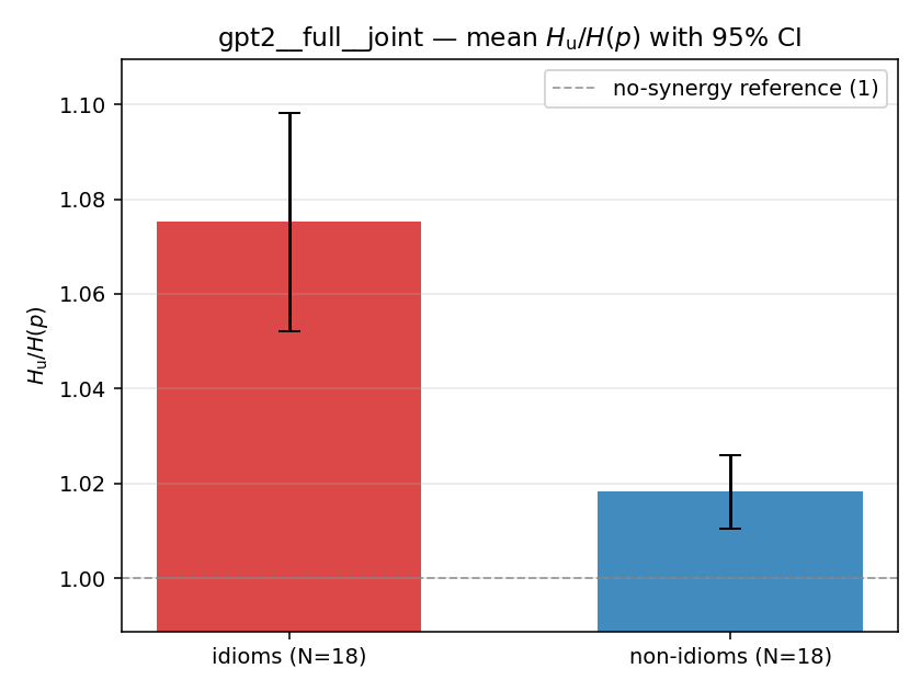 | 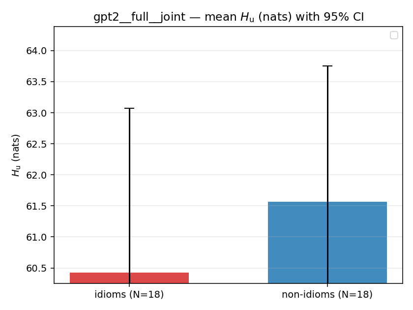 | 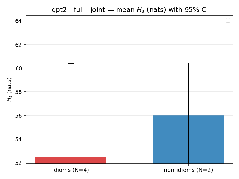 | 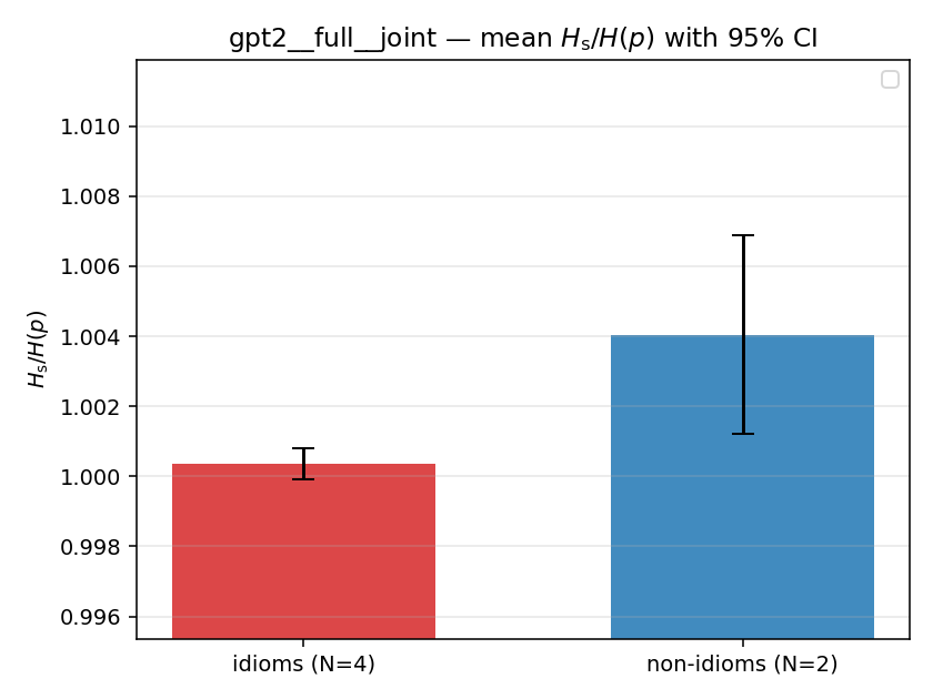 | 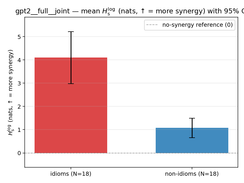 | 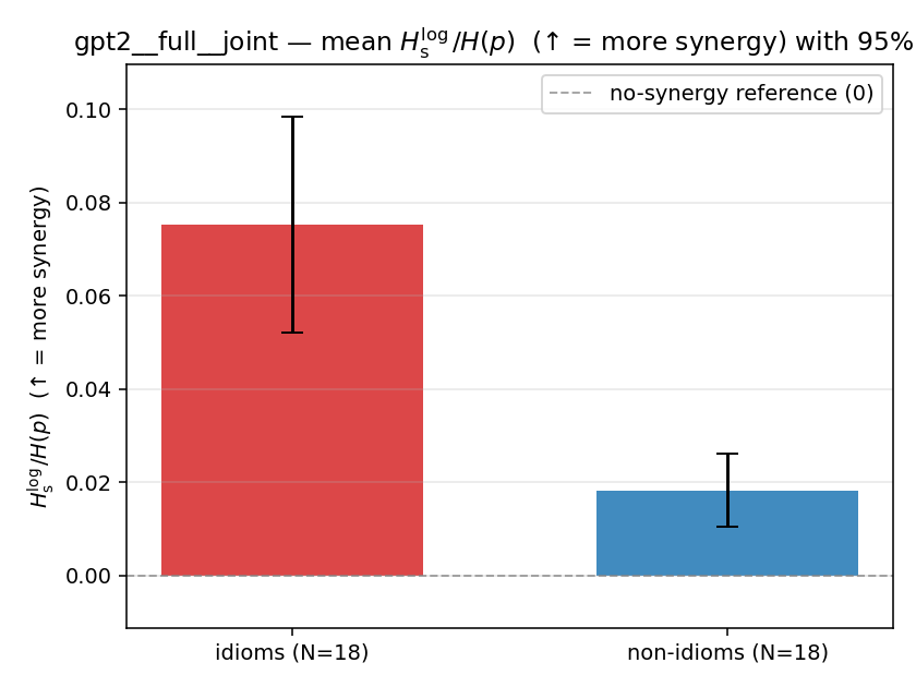 | 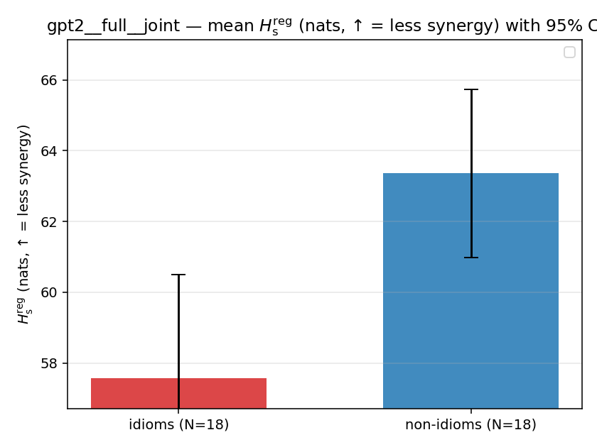 | 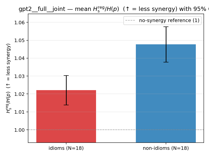 | 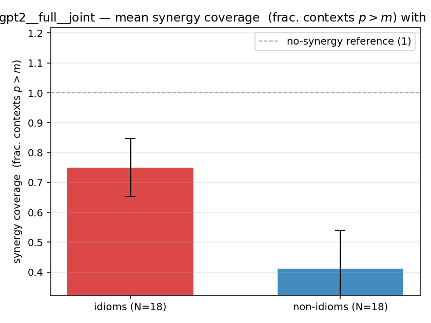 |
| per-idiom (sorted) | 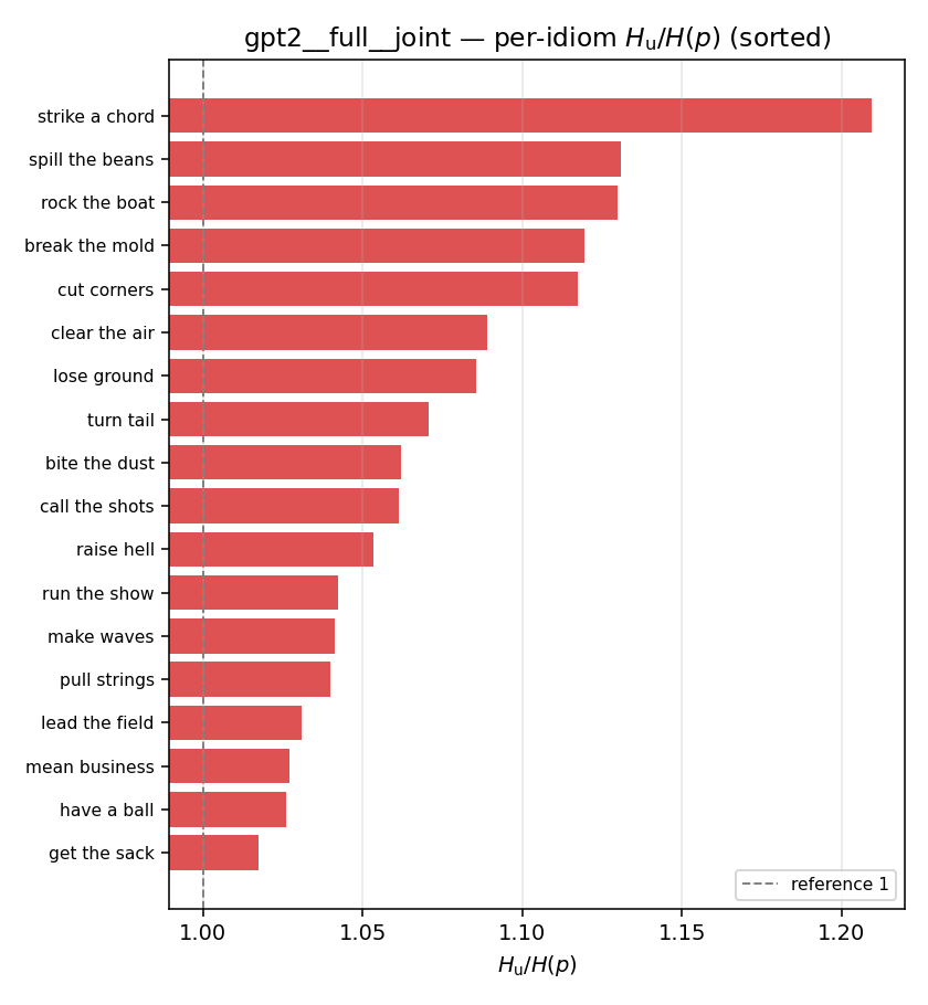 | 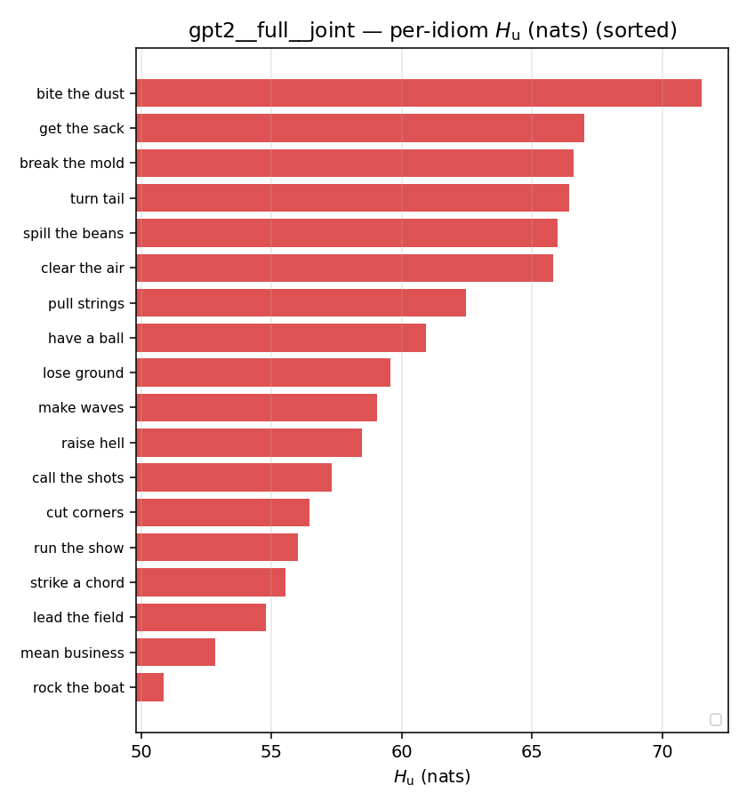 | 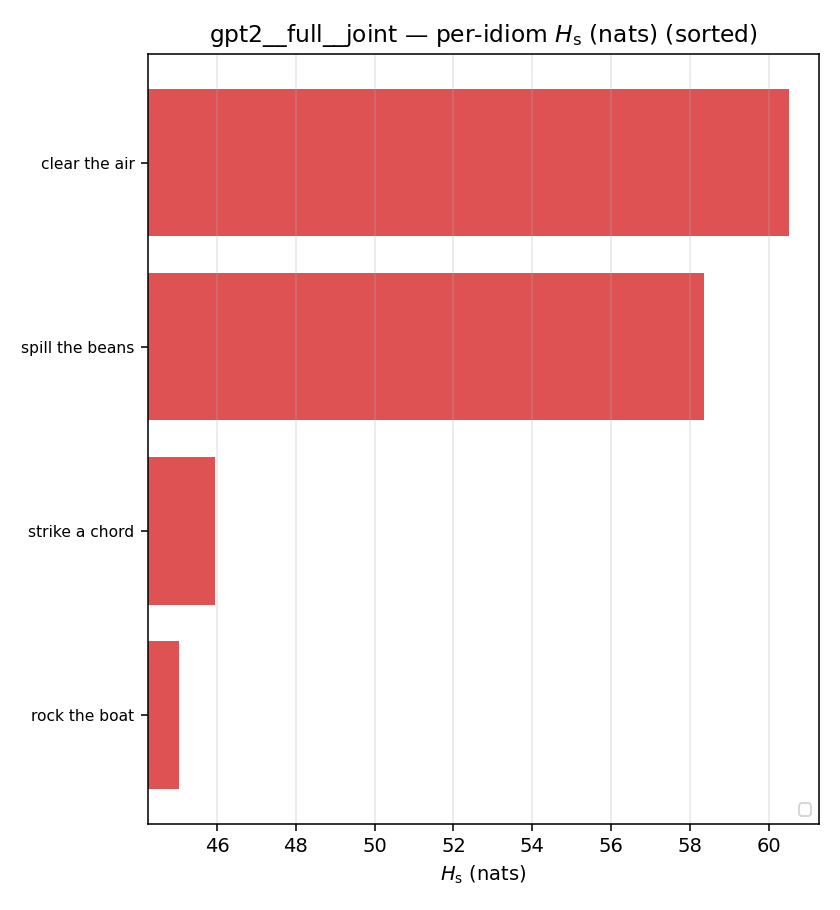 | 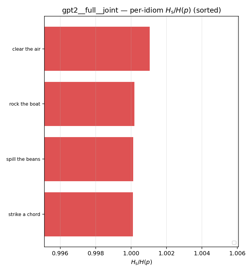 | 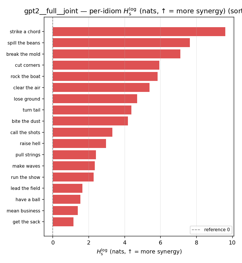 | 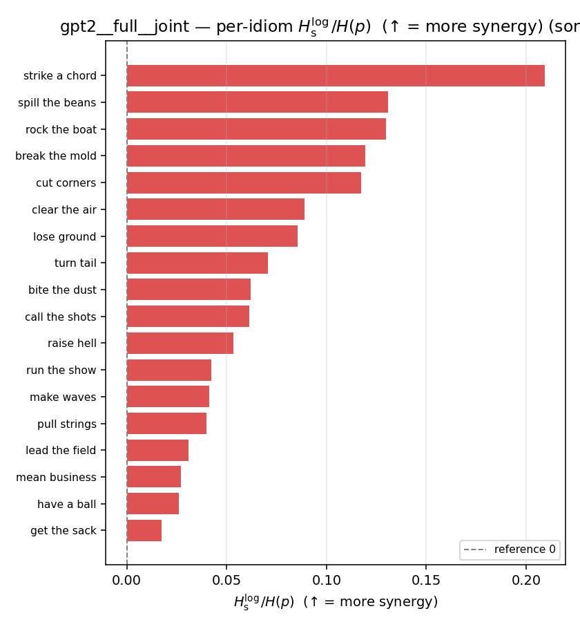 | 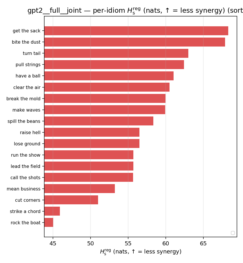 | 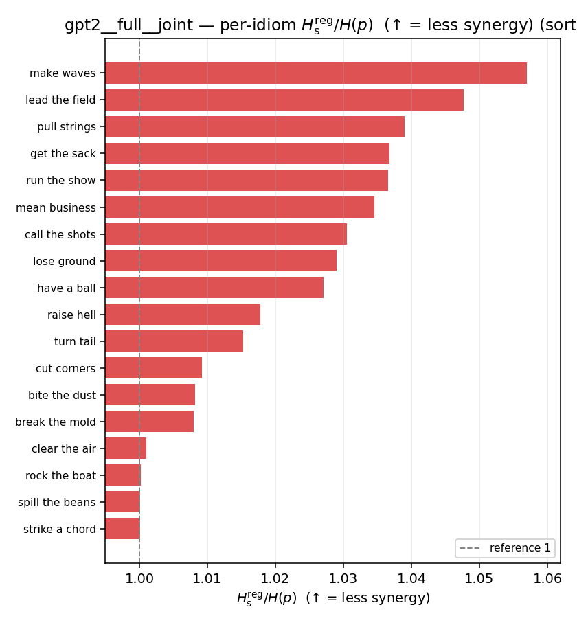 | 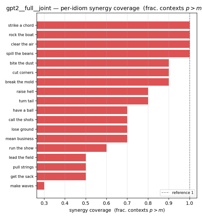 |
gemma2-9b — per-config figures
3×9 grid of figure-type × metric (↑syn / ↓syn in a header = the metric increases / decreases with synergy; definitions on the entropies page). Tables scroll horizontally; “— (no finite values)” marks Ĥs/ratio_s panels where every phrase was +inf. Click to zoom.
gemma2-9b · medial · geo gemma2-9b__medial__geo
| Ĥu/Ĥ ↑syn | Ĥu | Ĥs ↓syn | Ĥs/Ĥ ↓syn | Ĥslog ↑syn | Ĥslog/Ĥ ↑syn | Ĥsreg ↓syn | Ĥsreg/Ĥ ↓syn | f̂syn ↑syn | |
|---|---|---|---|---|---|---|---|---|---|
| strip (per-phrase) | 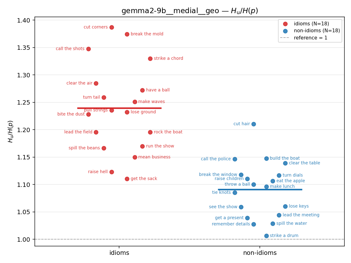 | 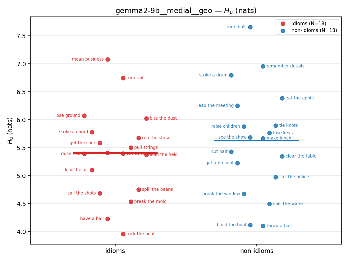 | 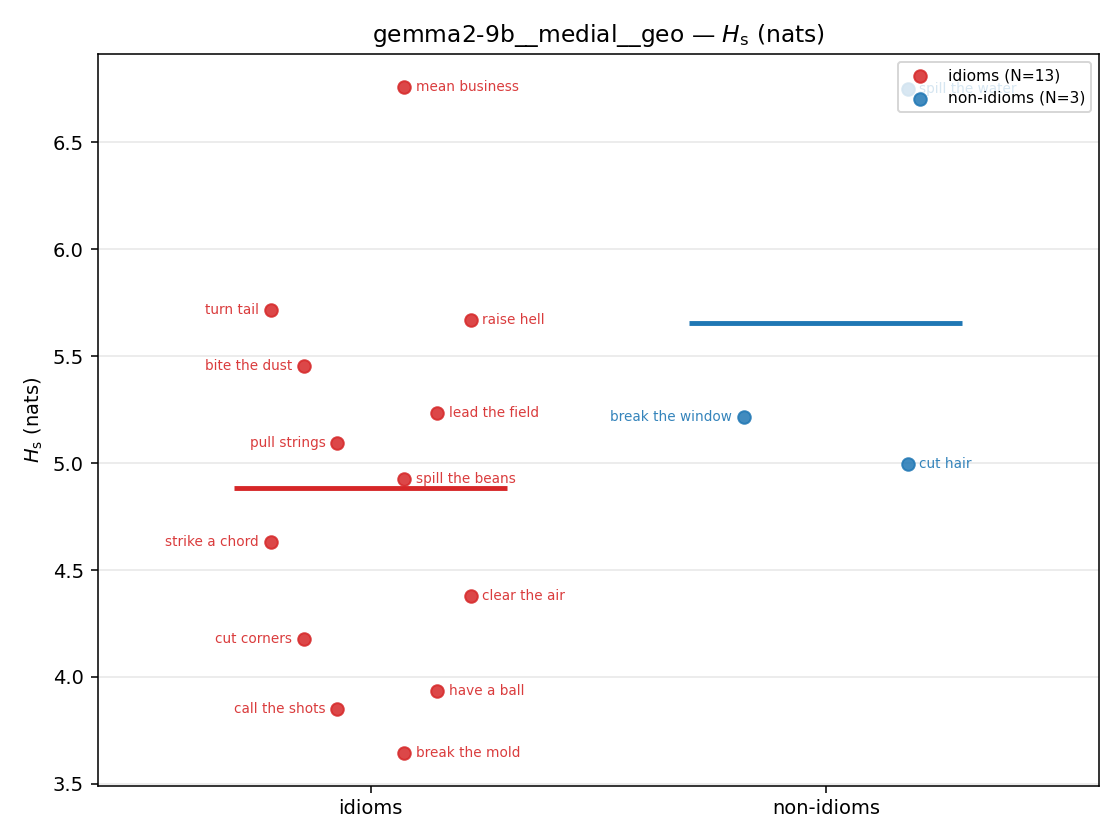 | 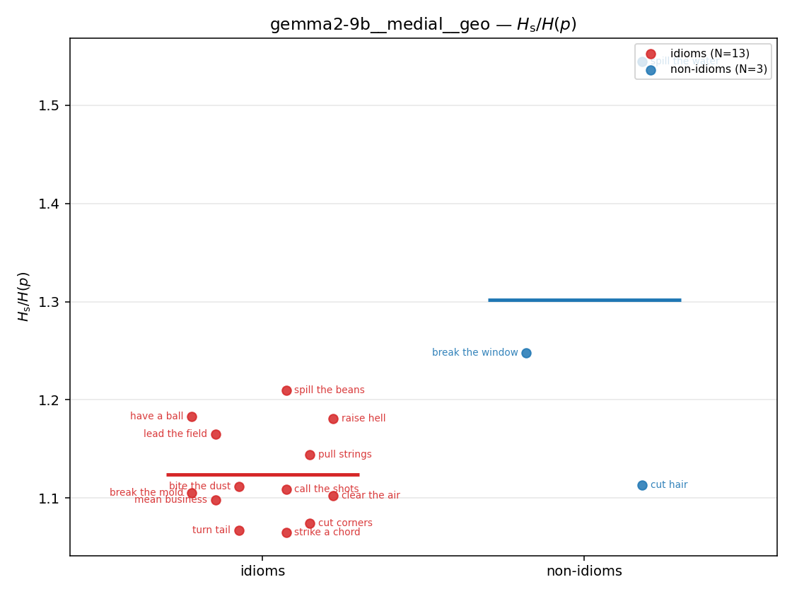 | 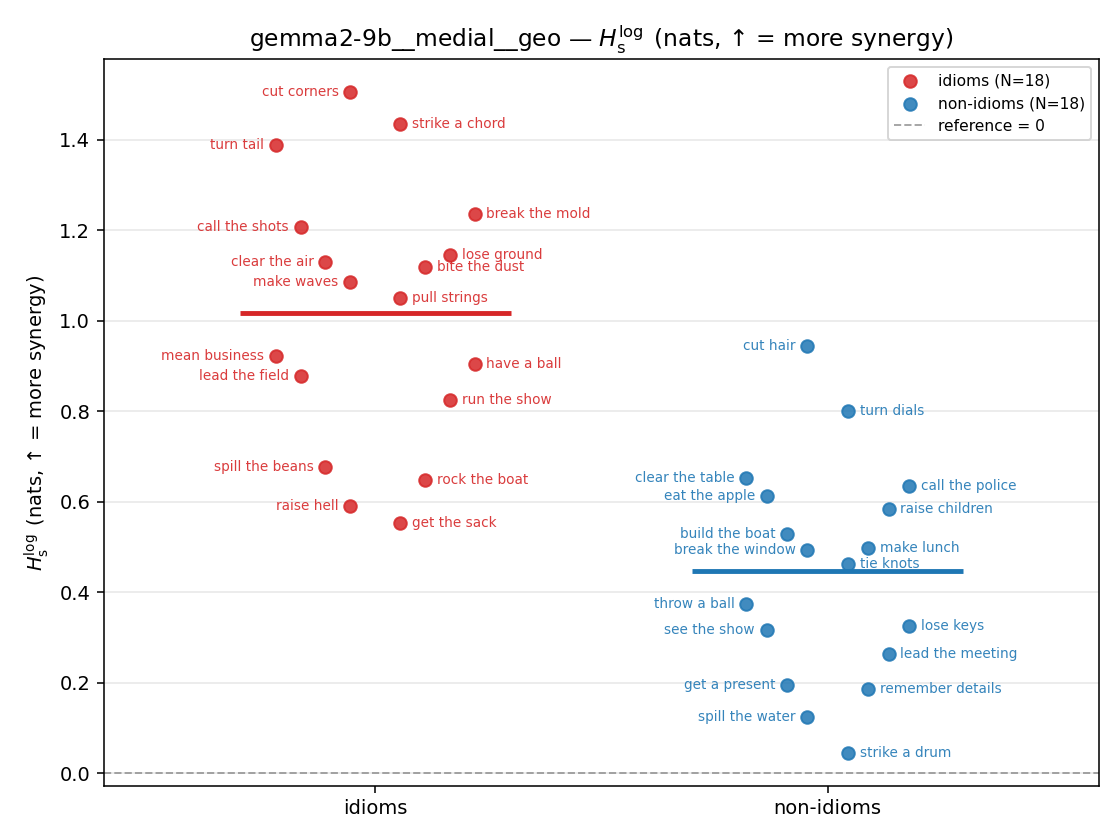 | 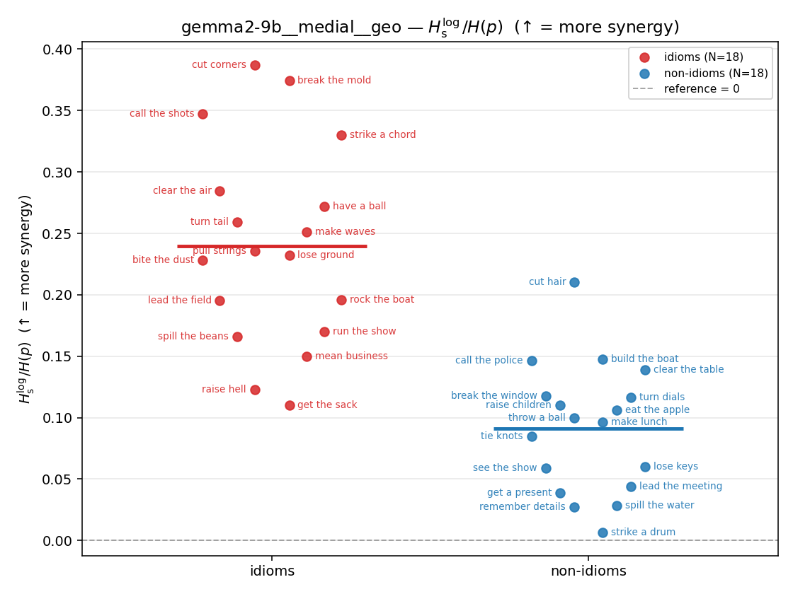 | 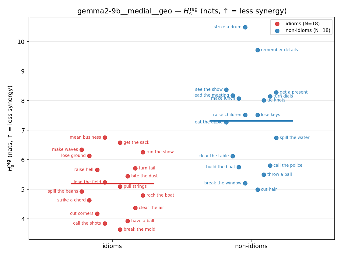 | 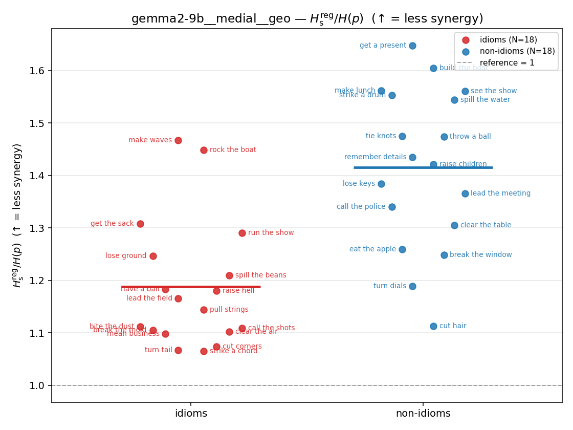 | 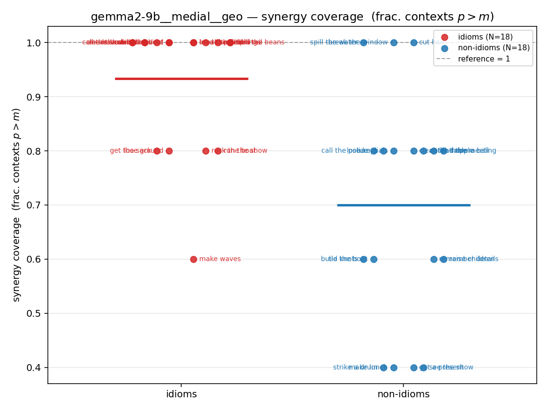 |
| mean ± 95% CI | 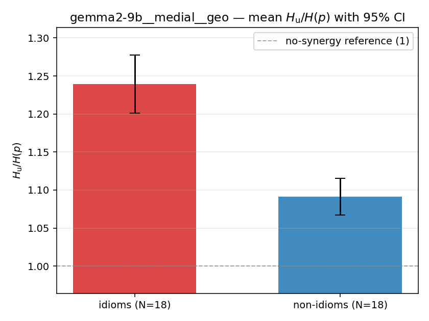 | 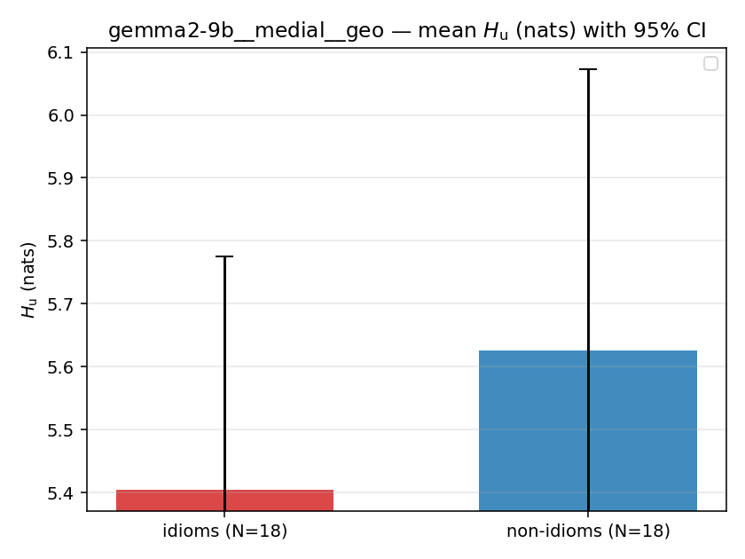 | 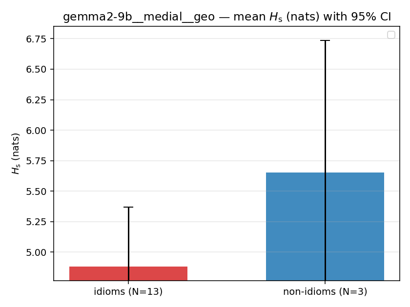 | 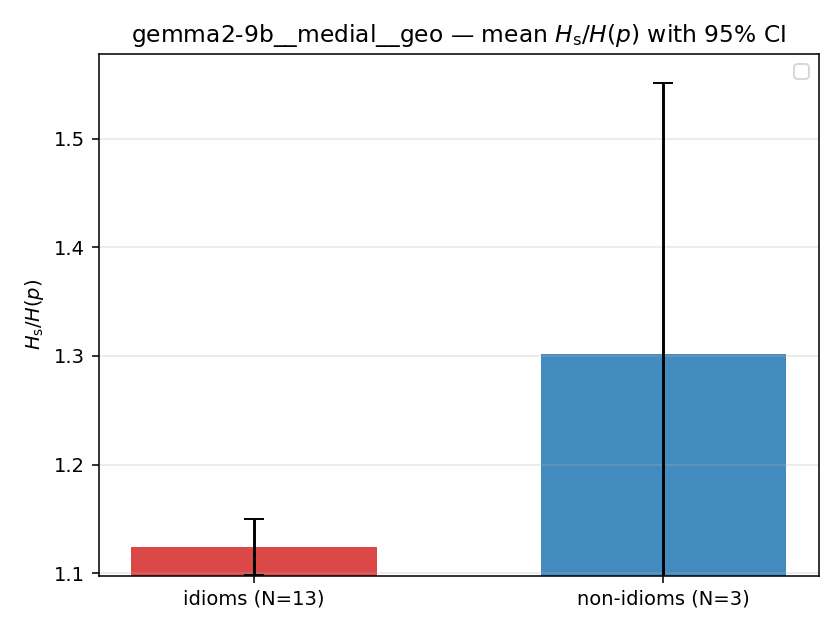 | 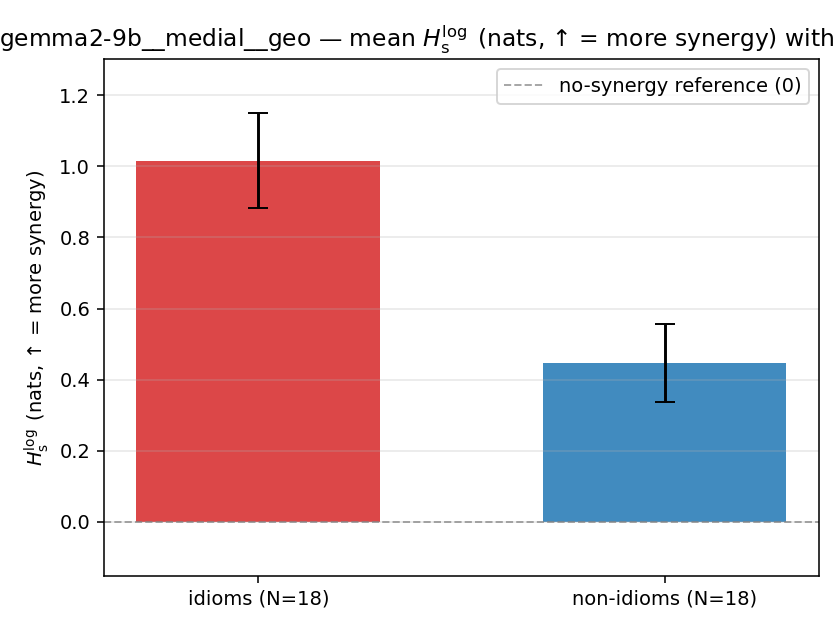 | 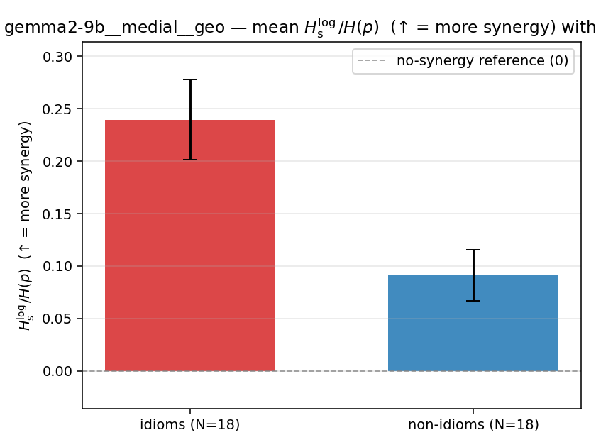 | 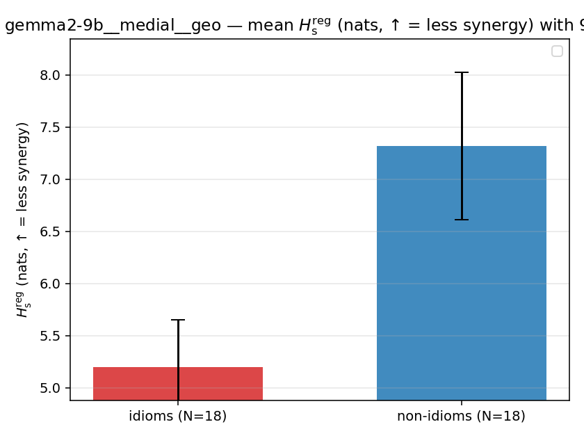 | 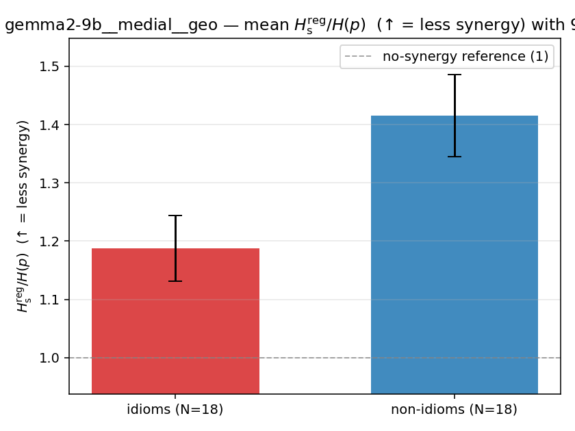 | 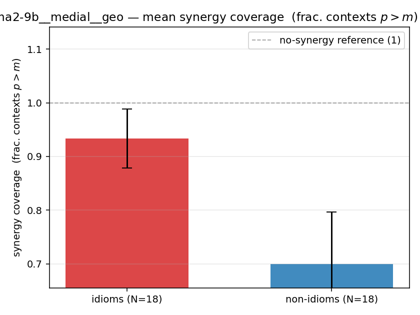 |
| per-idiom (sorted) | 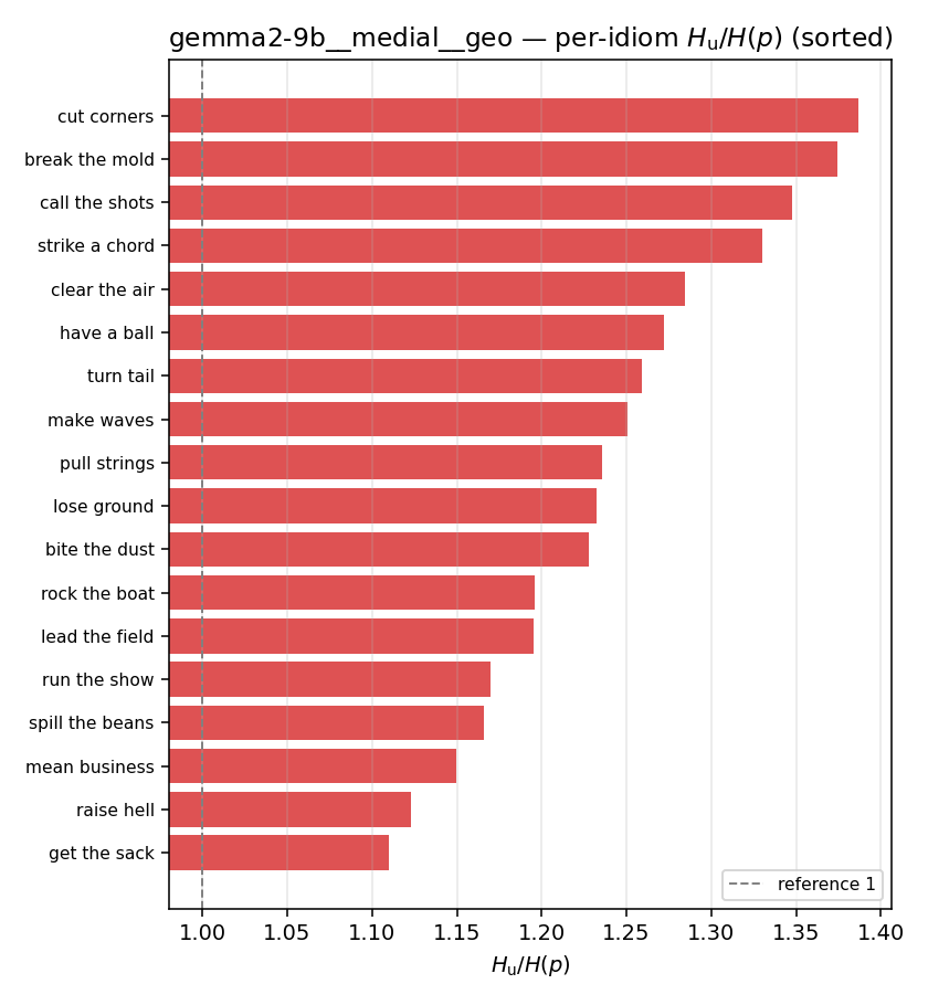 | 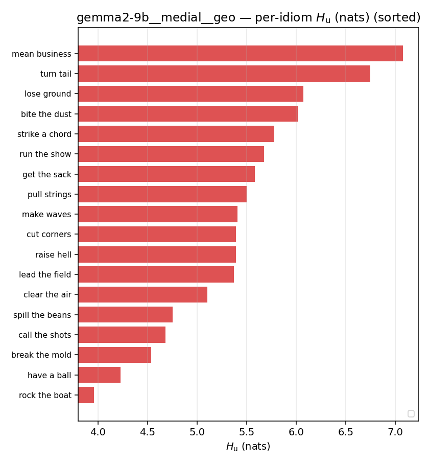 | 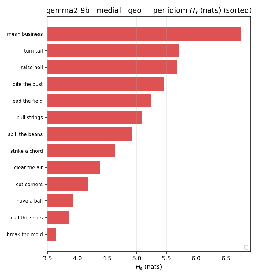 | 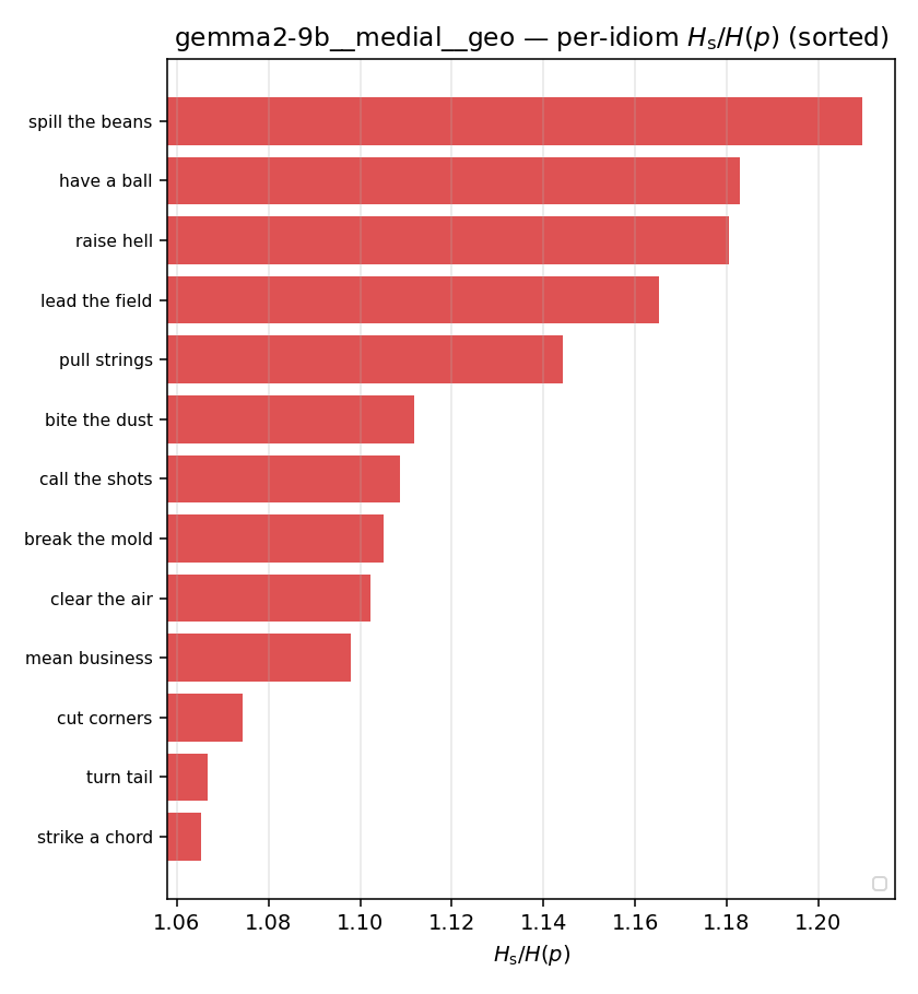 | 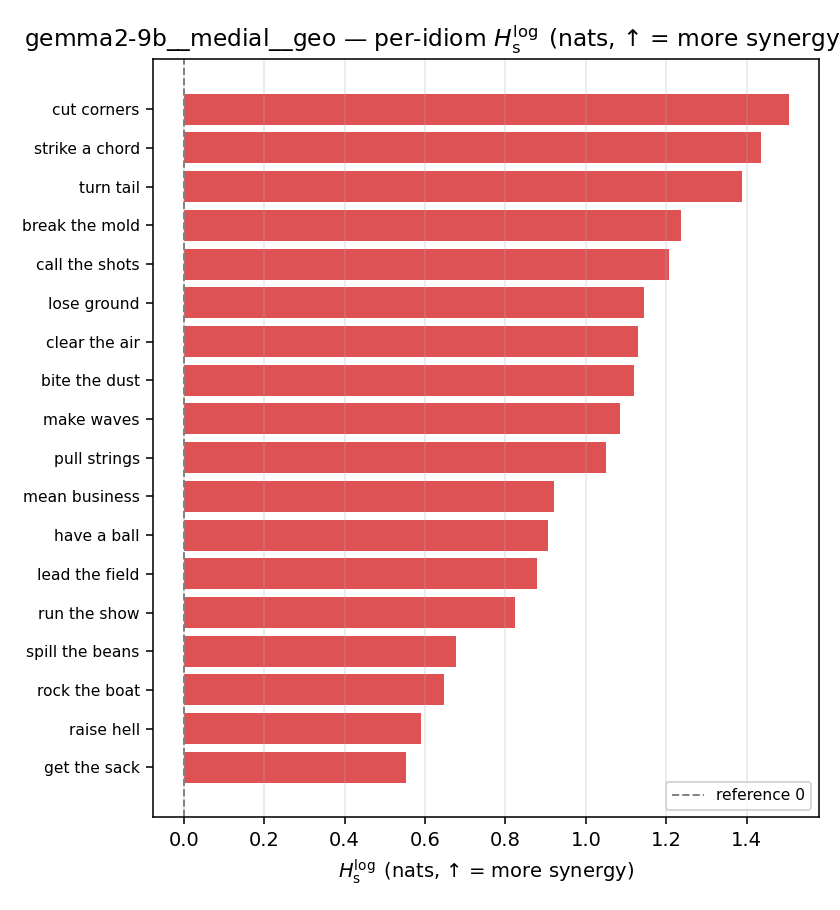 | 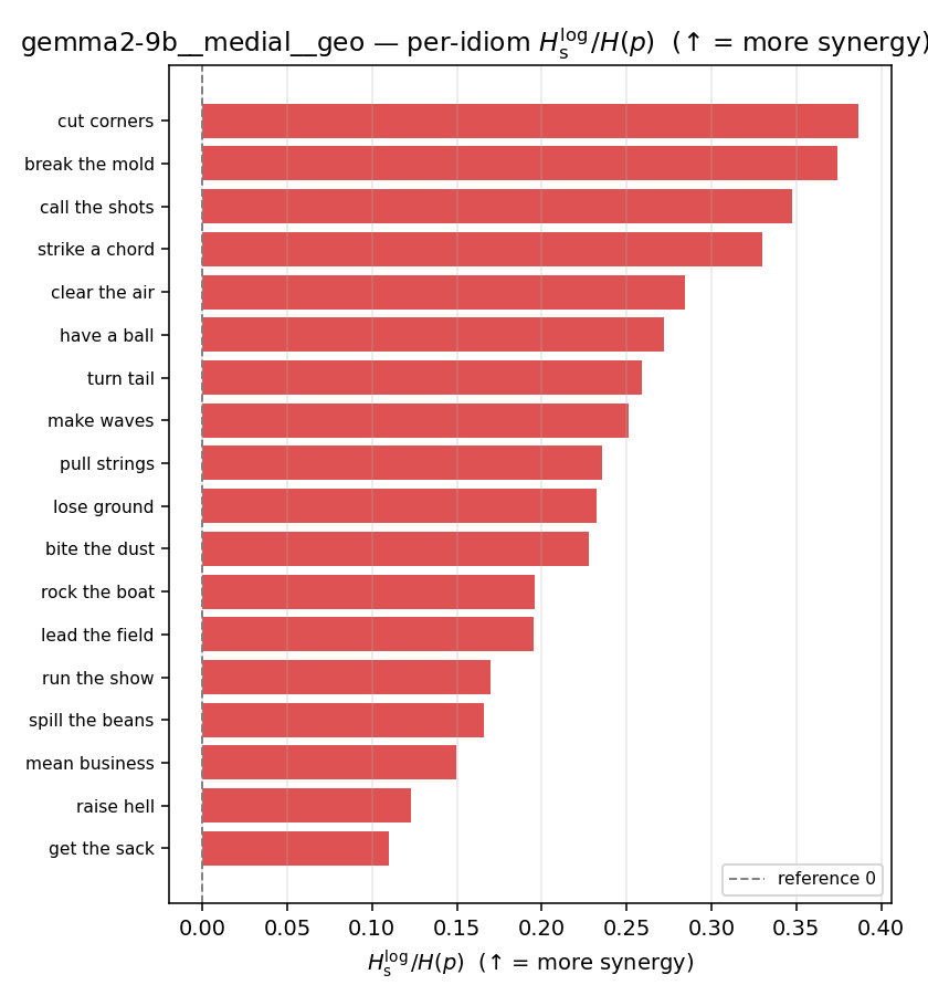 | 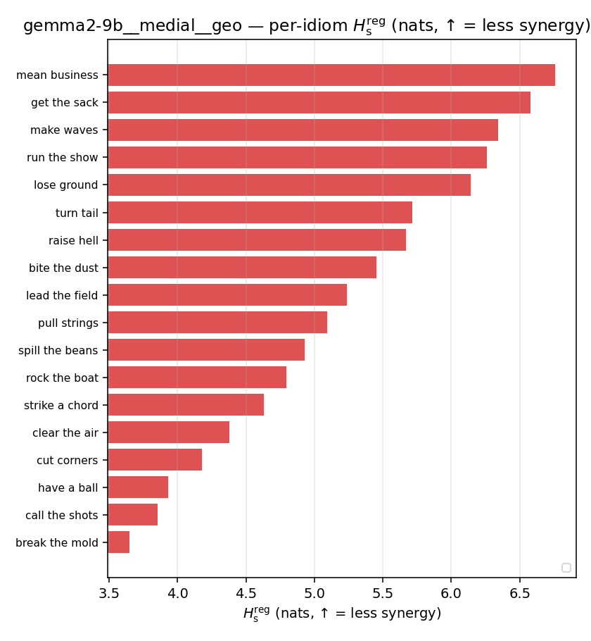 | 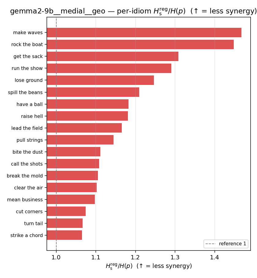 | 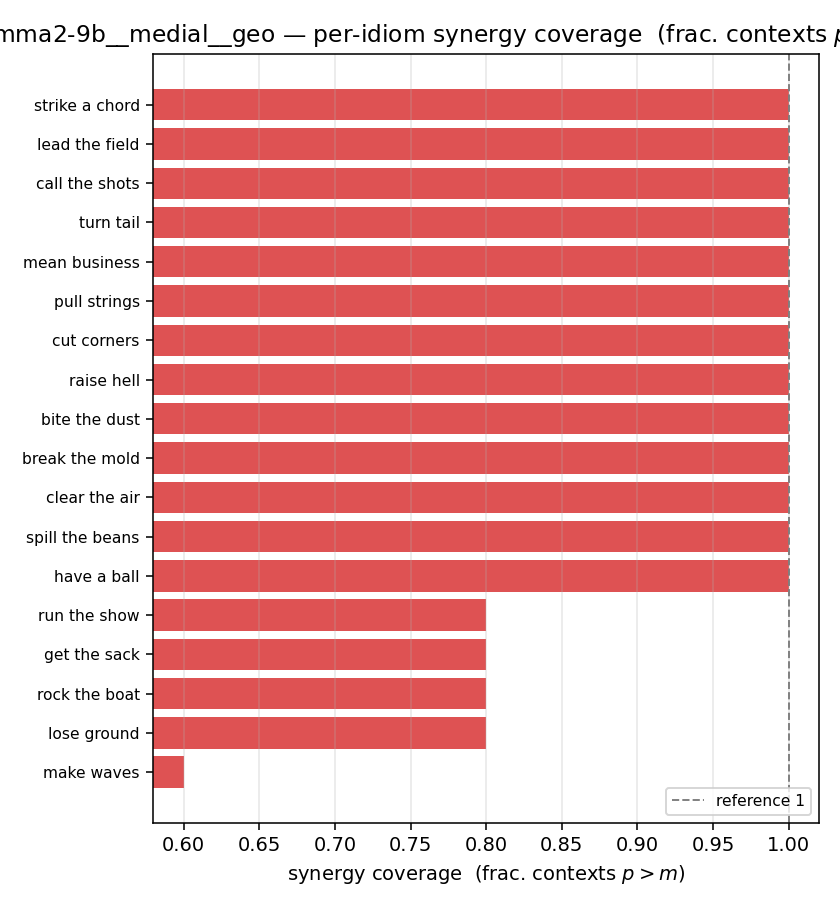 |
gemma2-9b · medial · joint gemma2-9b__medial__joint
| Ĥu/Ĥ ↑syn | Ĥu | Ĥs ↓syn | Ĥs/Ĥ ↓syn | Ĥslog ↑syn | Ĥslog/Ĥ ↑syn | Ĥsreg ↓syn | Ĥsreg/Ĥ ↓syn | f̂syn ↑syn | |
|---|---|---|---|---|---|---|---|---|---|
| strip (per-phrase) | 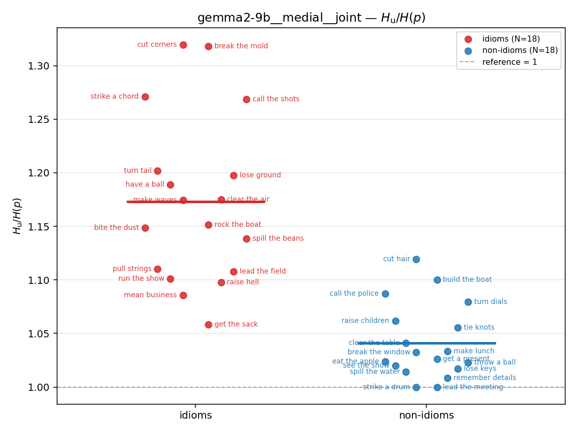 | 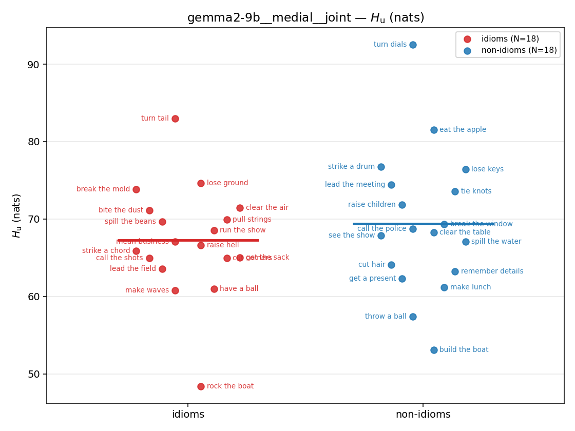 | 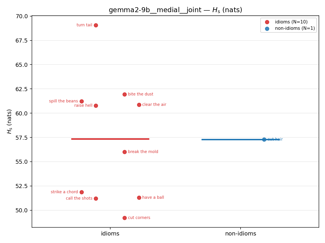 | 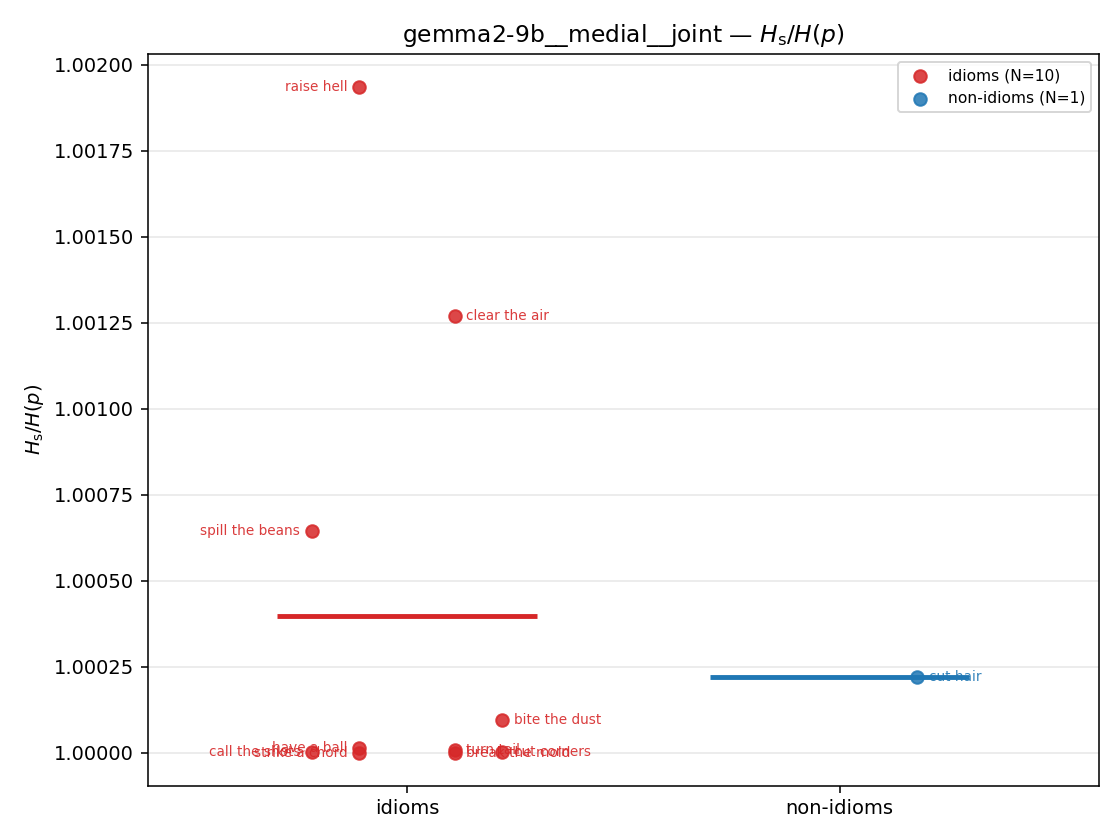 | 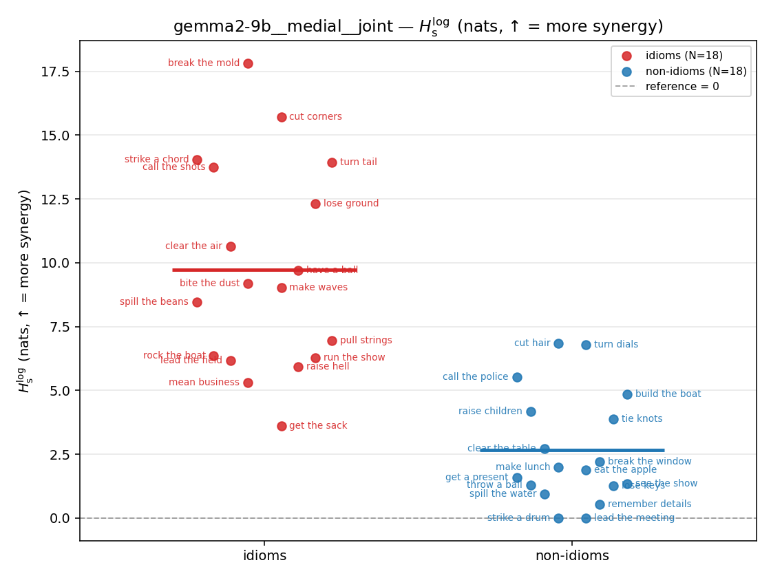 | 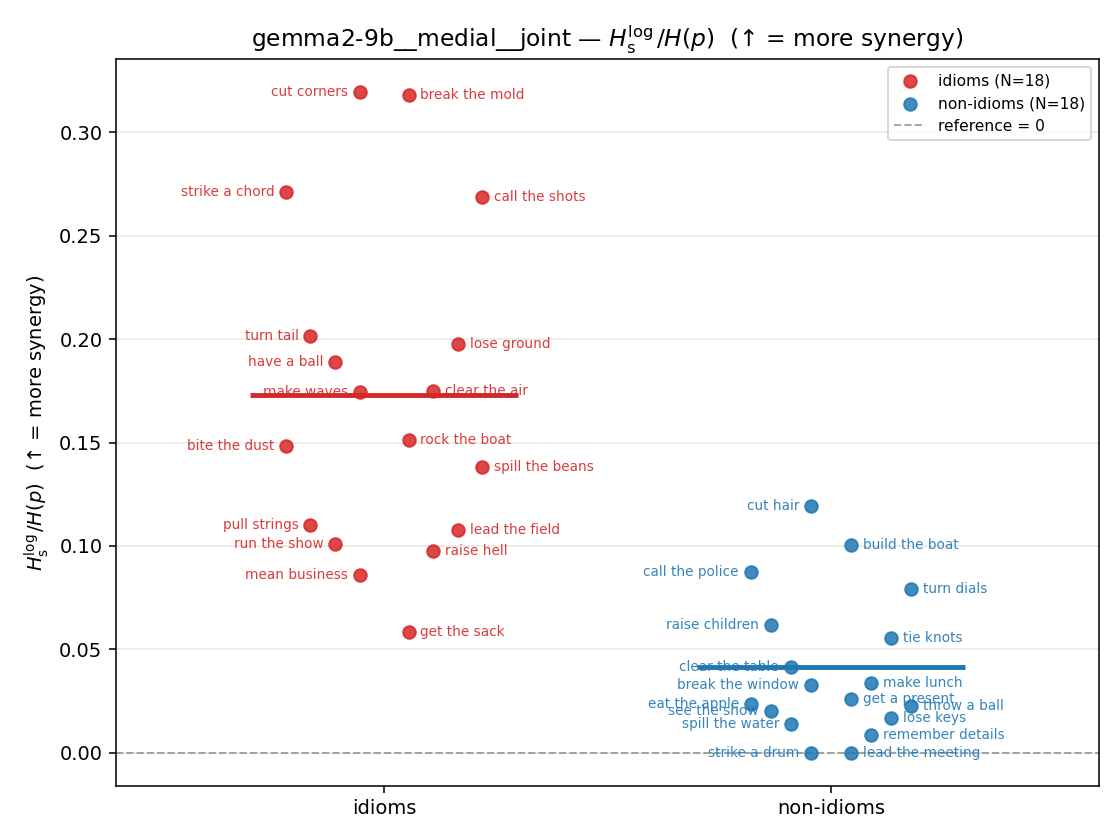 | 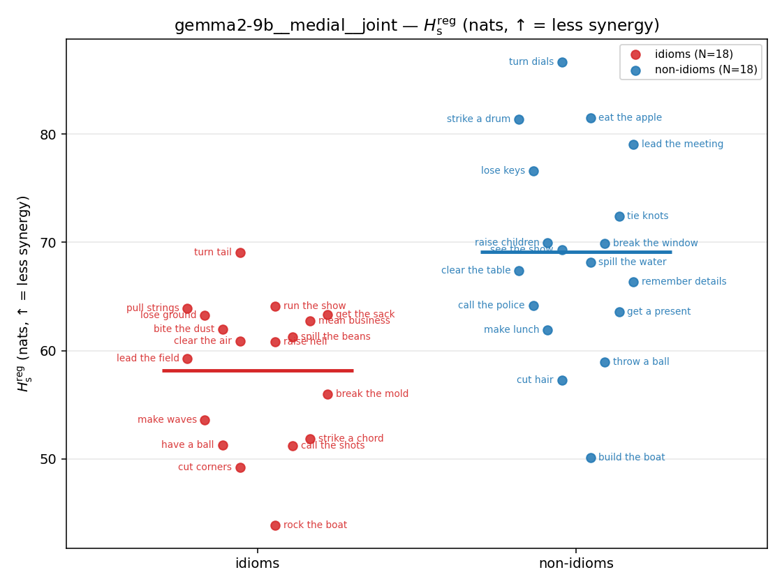 | 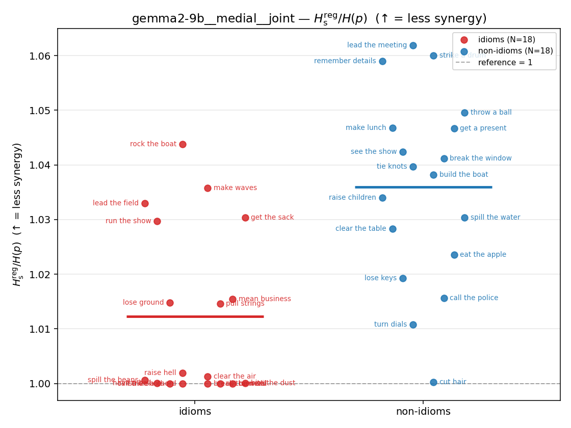 | 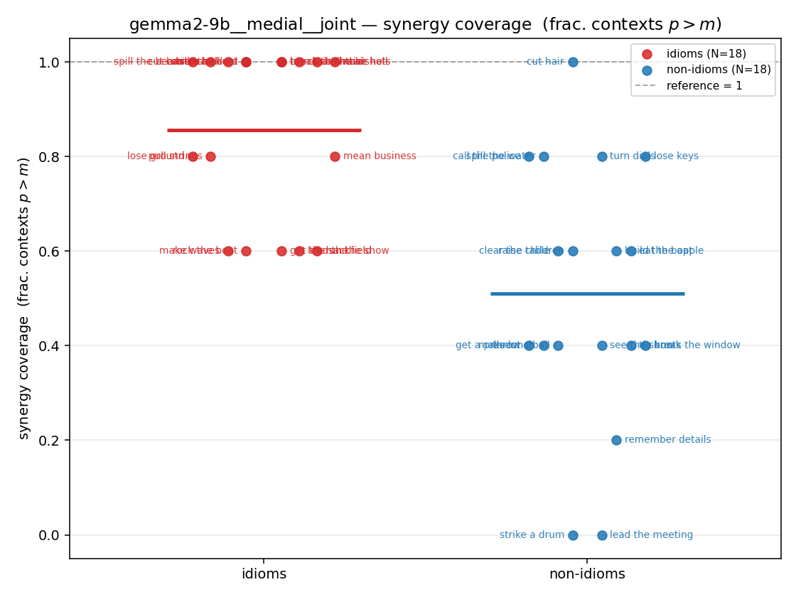 |
| mean ± 95% CI | 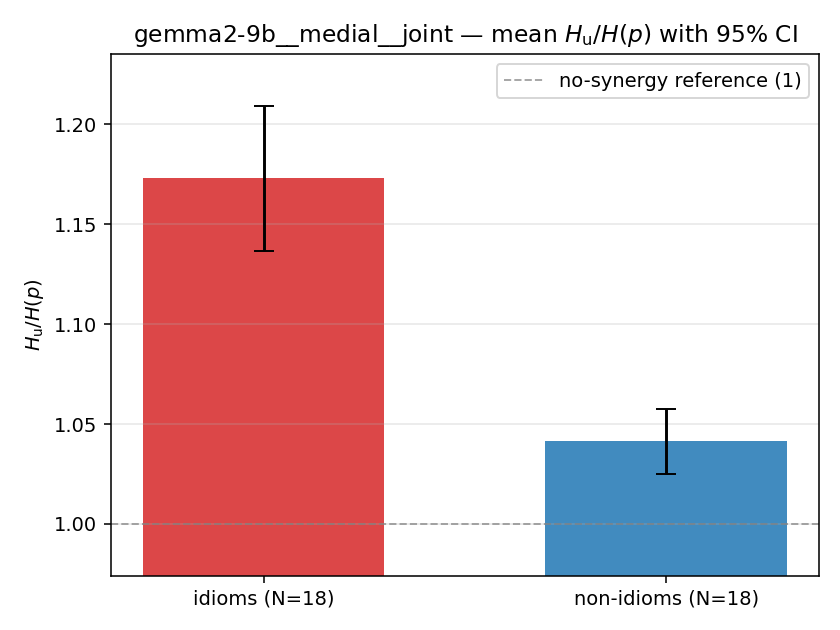 | 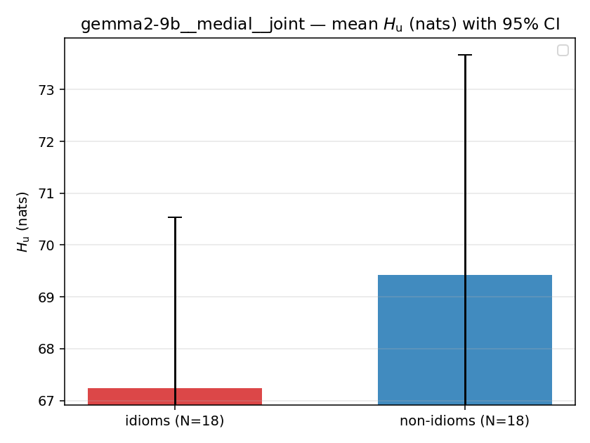 | 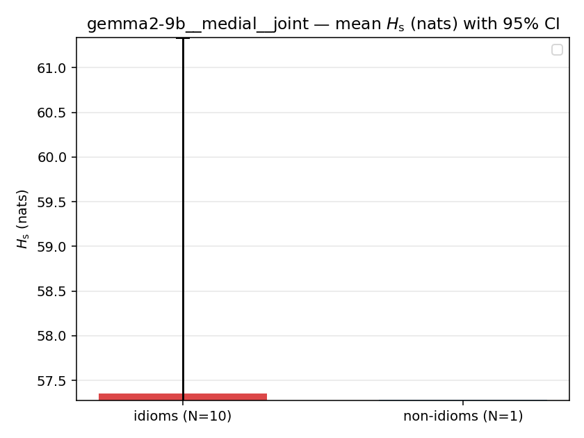 | 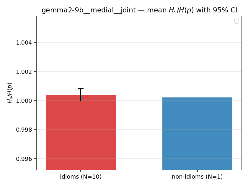 | 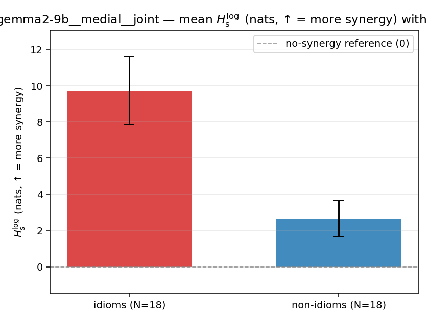 | 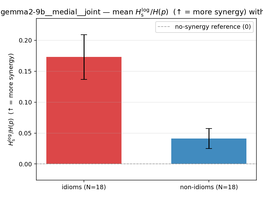 | 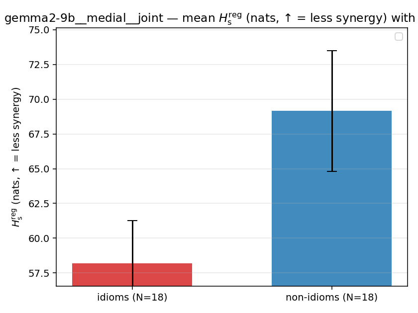 | 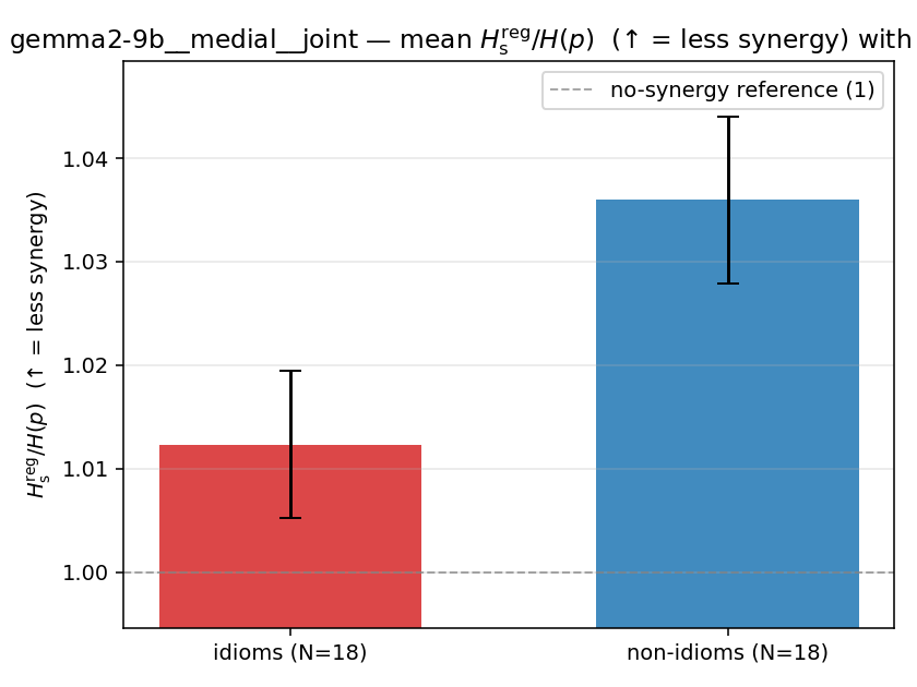 | 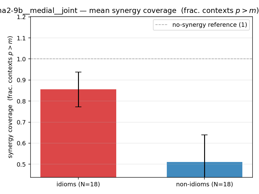 |
| per-idiom (sorted) | 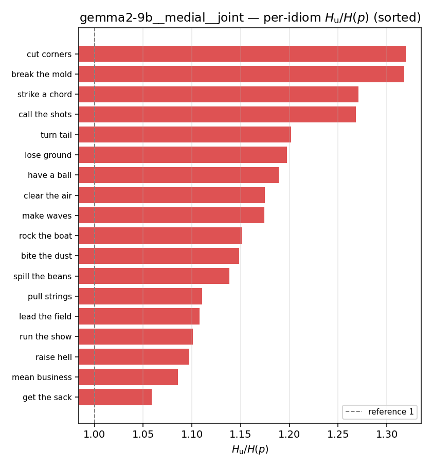 | 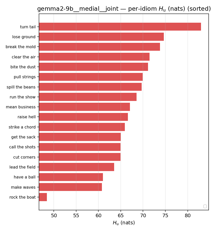 | 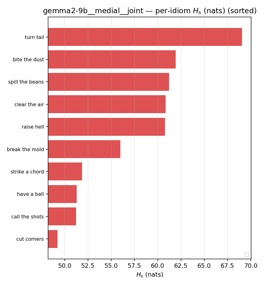 | 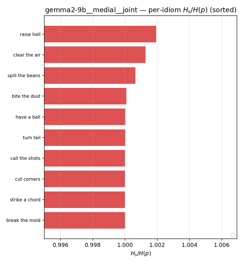 | 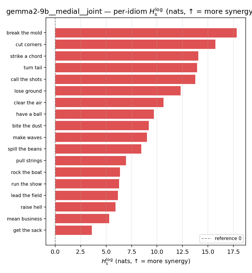 | 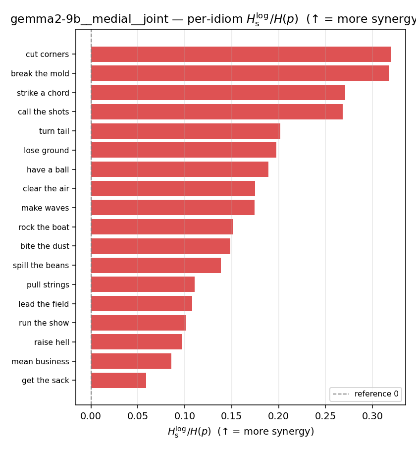 | 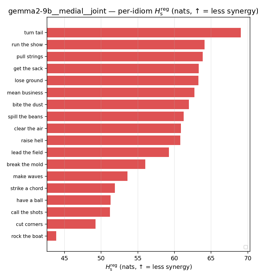 | 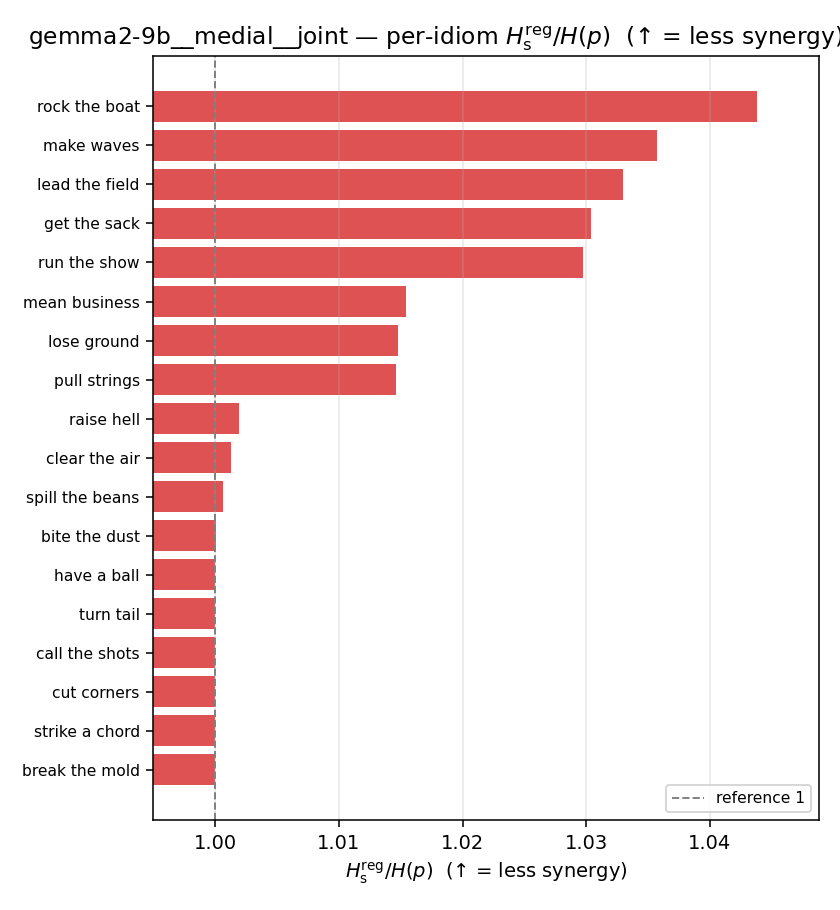 | 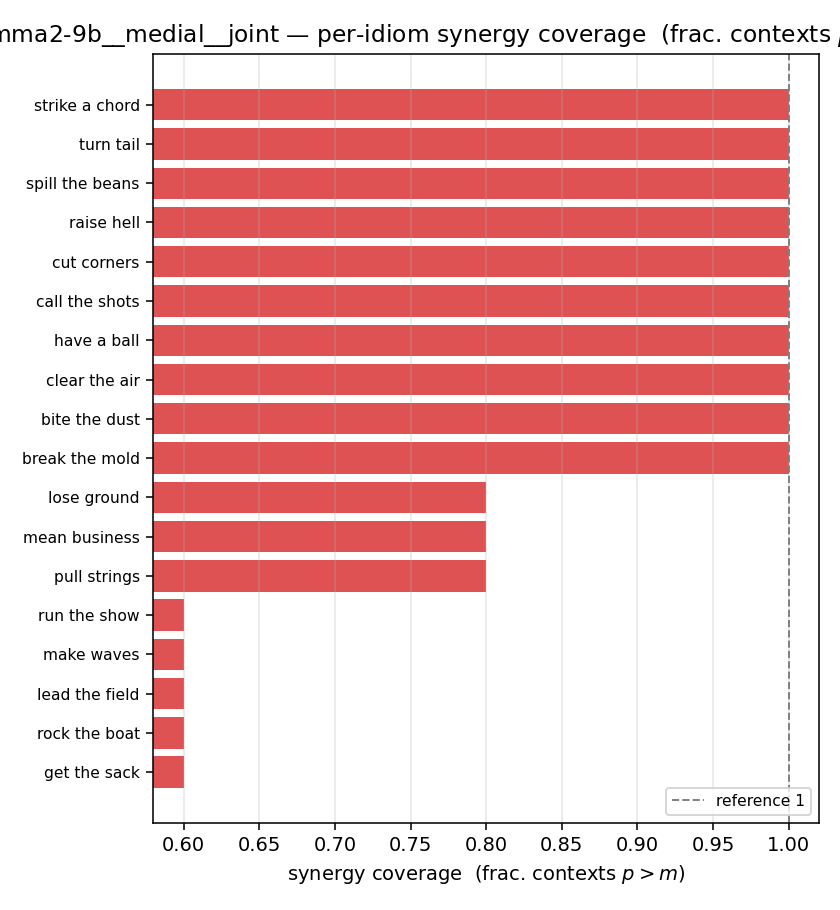 |
gemma2-9b · full · geo gemma2-9b__full__geo
| Ĥu/Ĥ ↑syn | Ĥu | Ĥs ↓syn | Ĥs/Ĥ ↓syn | Ĥslog ↑syn | Ĥslog/Ĥ ↑syn | Ĥsreg ↓syn | Ĥsreg/Ĥ ↓syn | f̂syn ↑syn | |
|---|---|---|---|---|---|---|---|---|---|
| strip (per-phrase) | 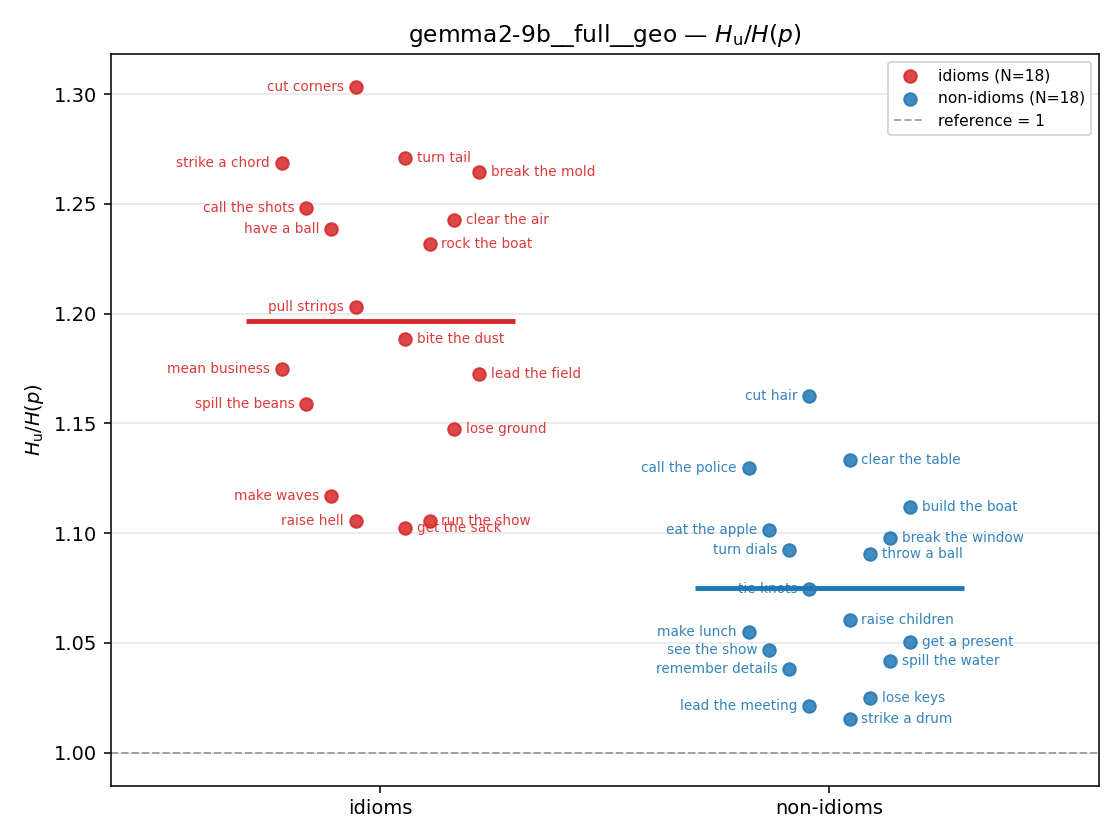 | 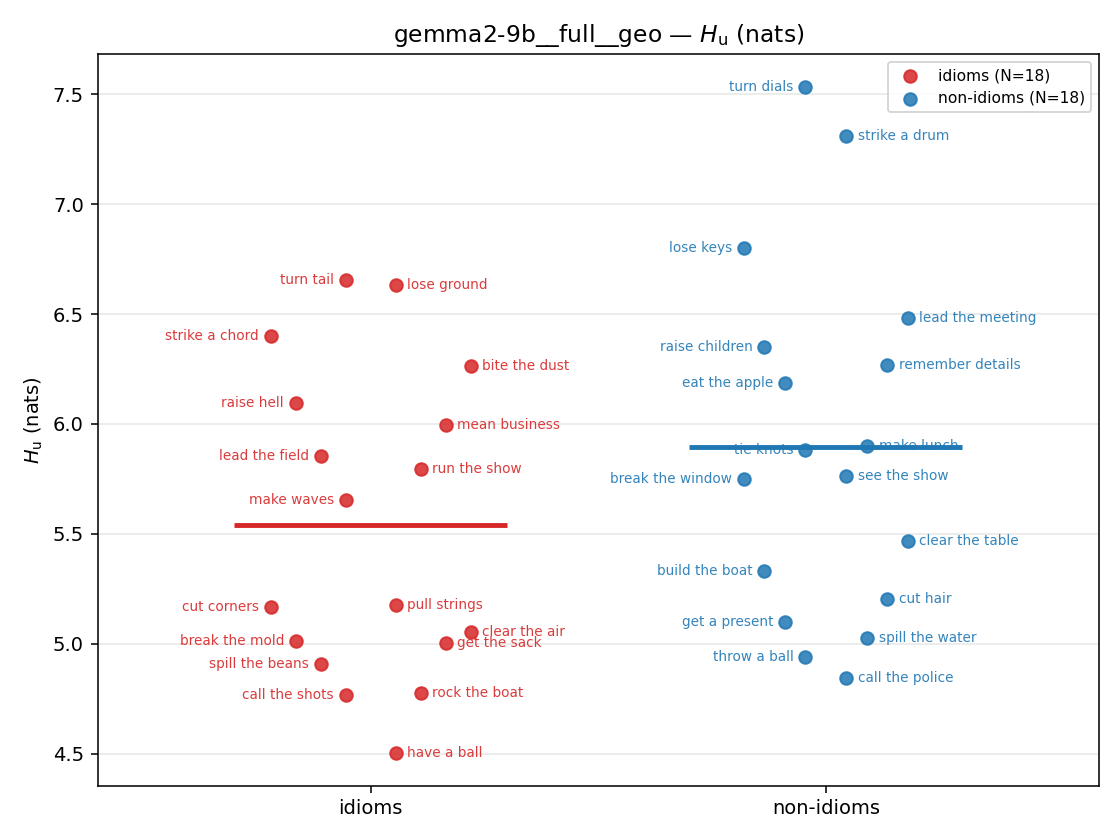 | 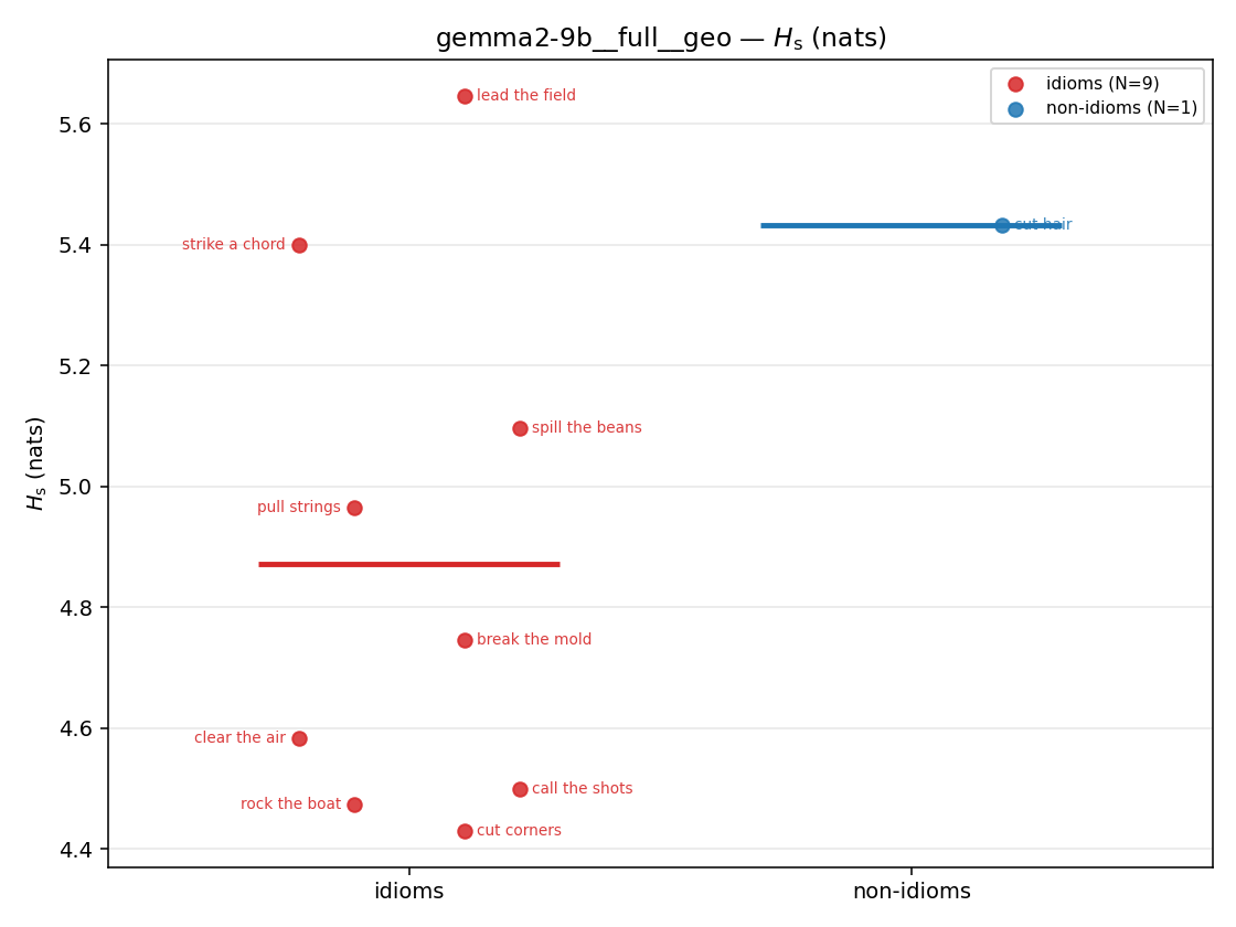 | 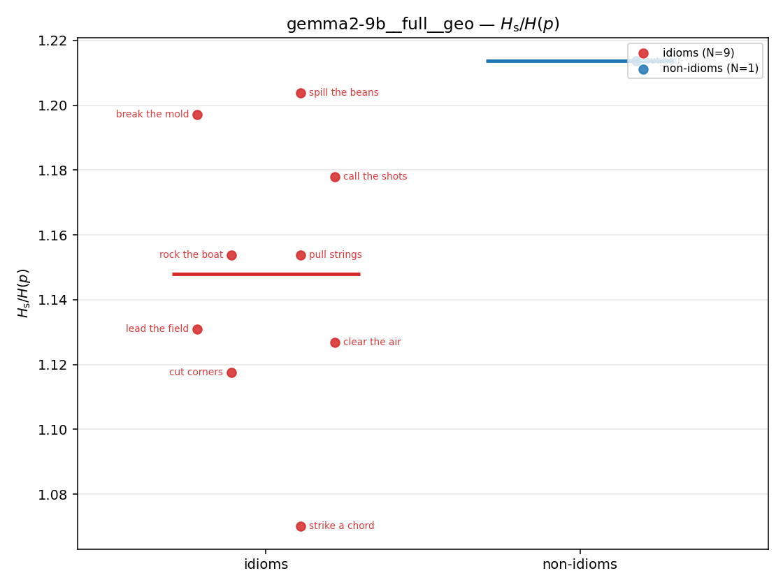 | 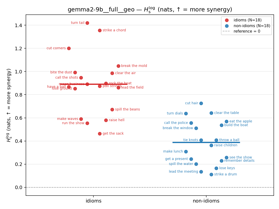 | 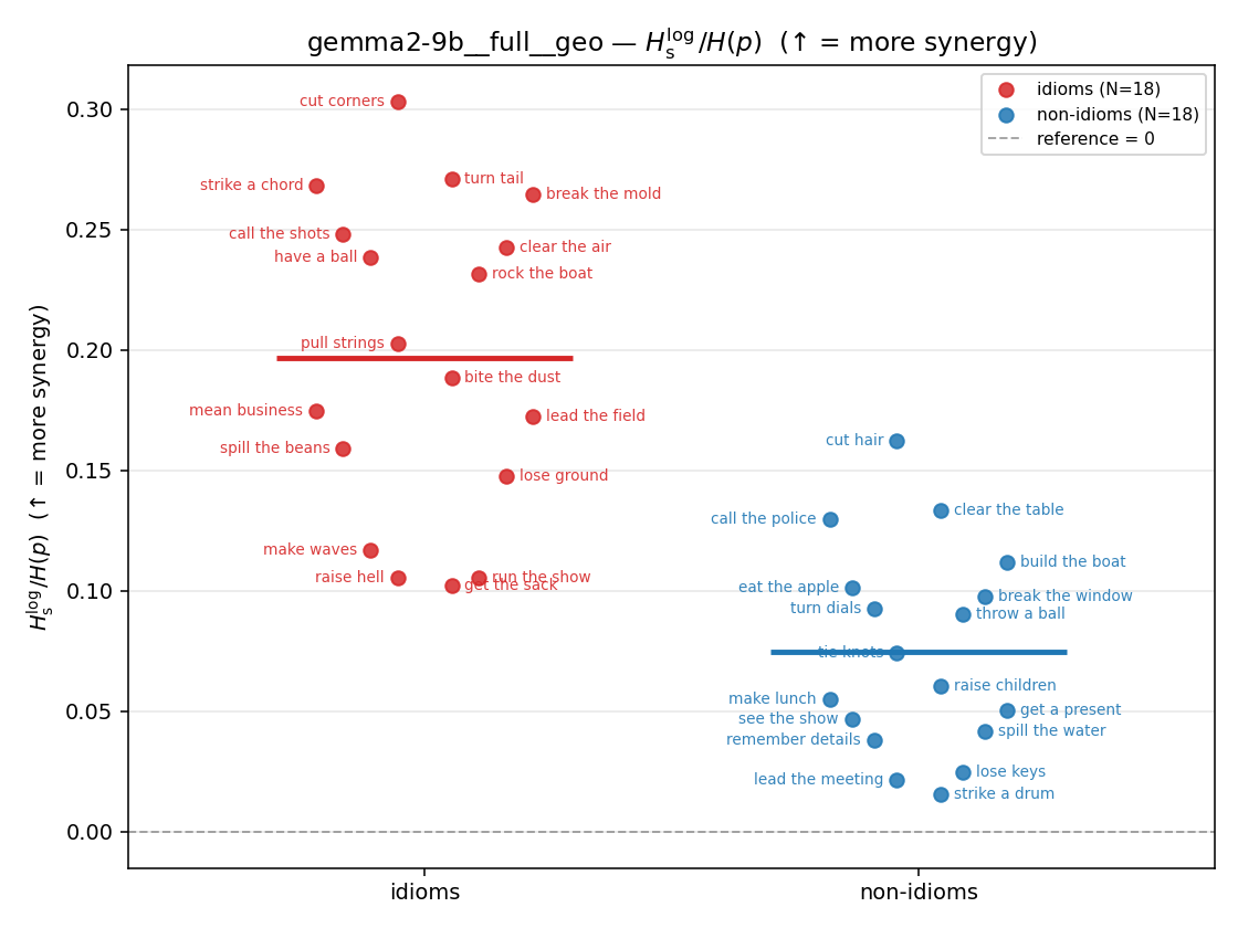 | 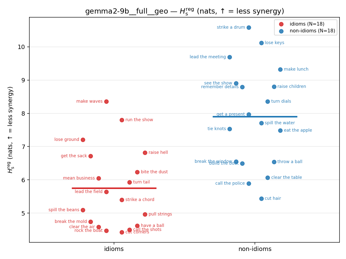 | 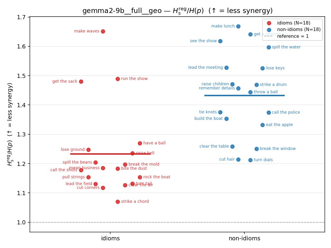 | 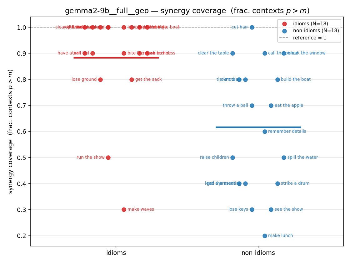 |
| mean ± 95% CI | 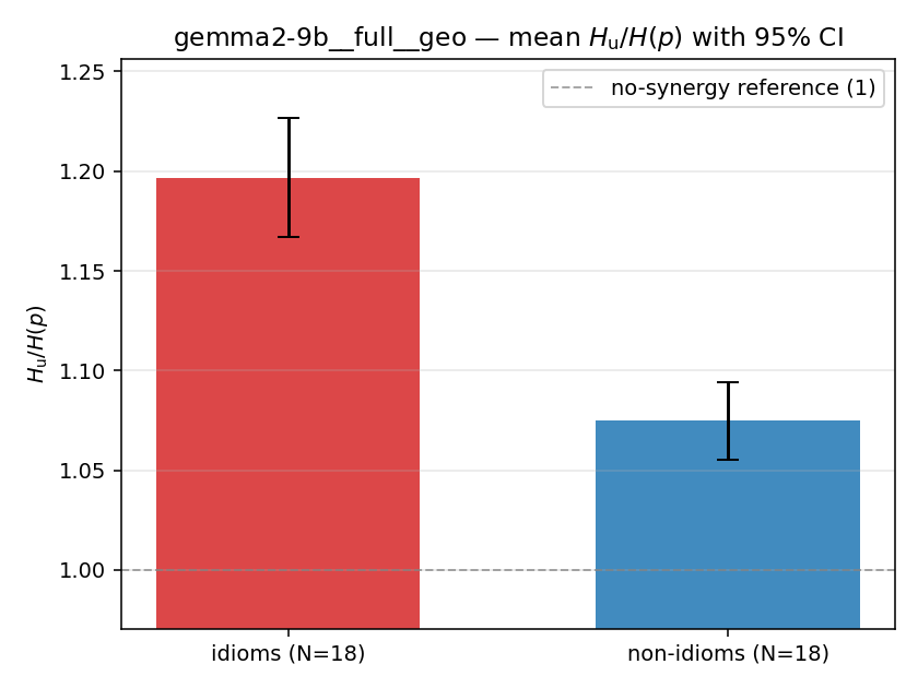 | 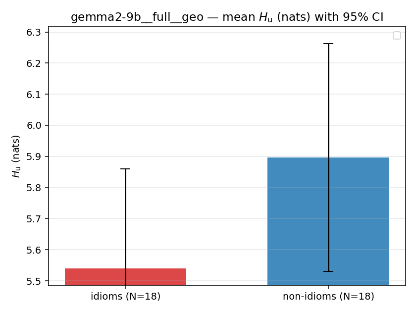 | 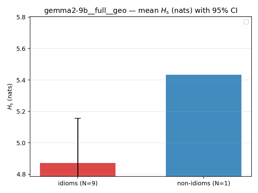 | 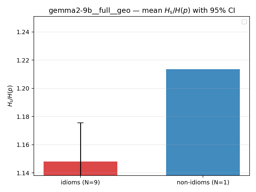 | 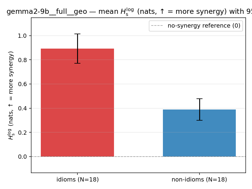 | 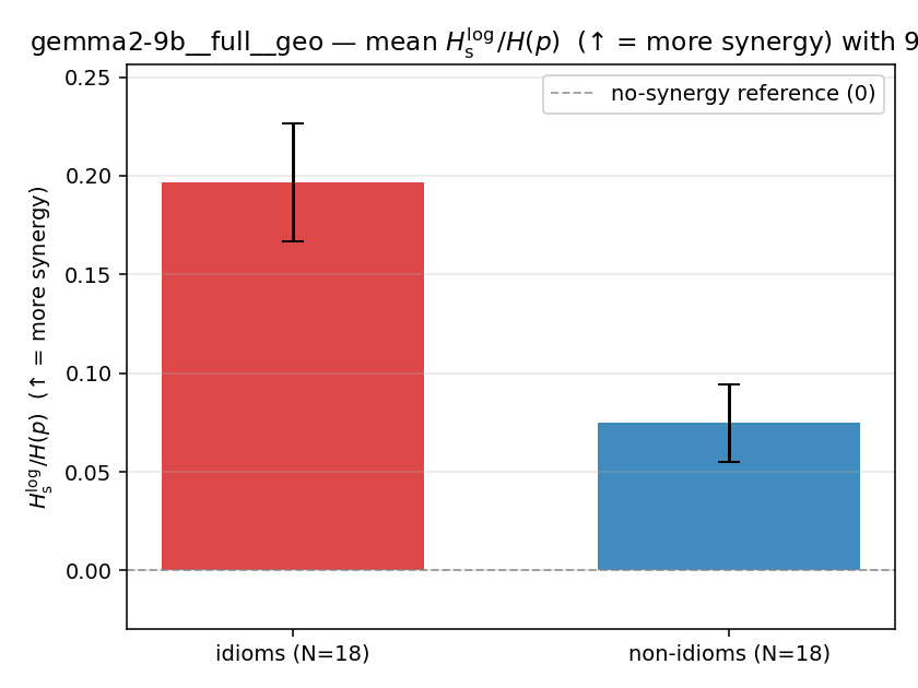 | 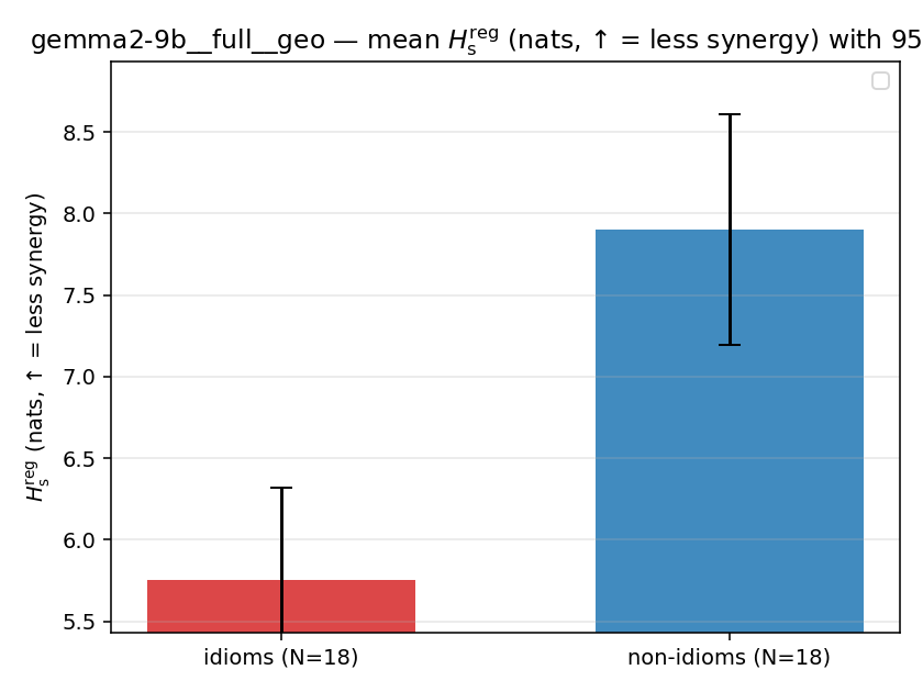 | 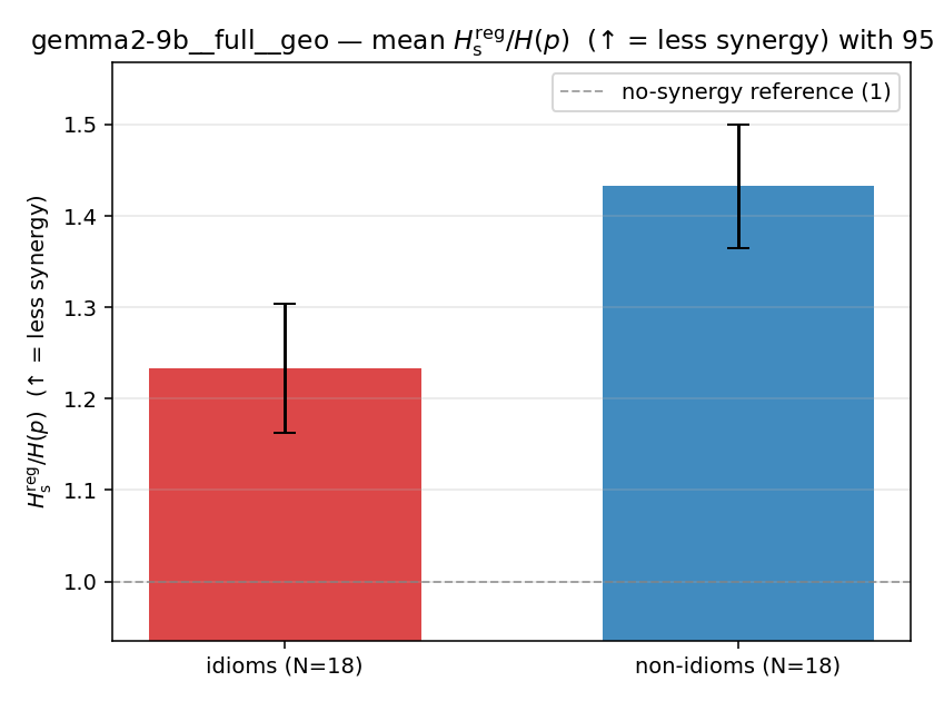 | 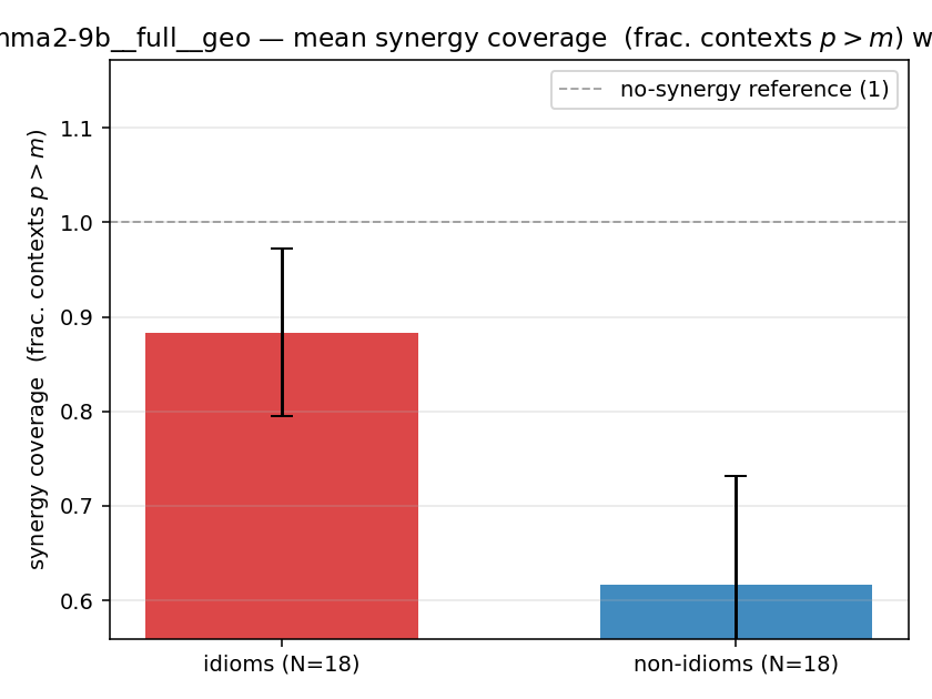 |
| per-idiom (sorted) | 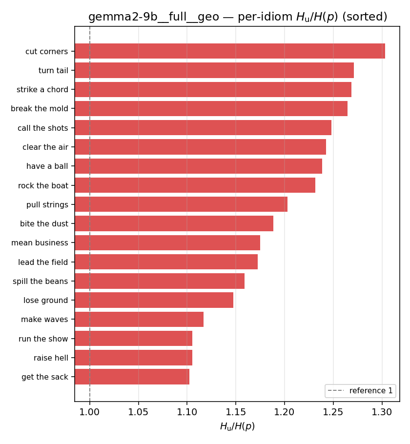 | 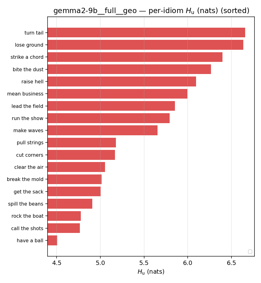 | 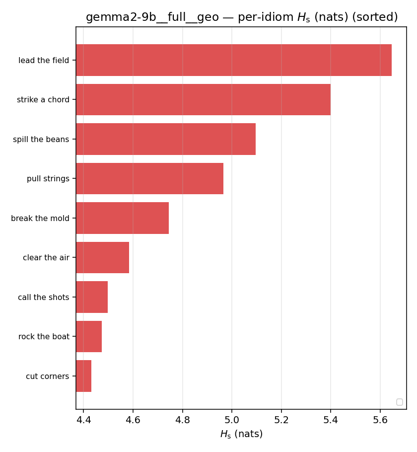 | 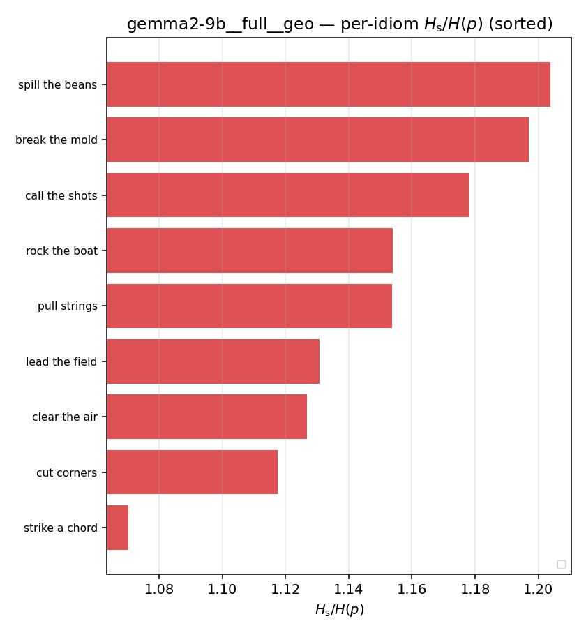 | 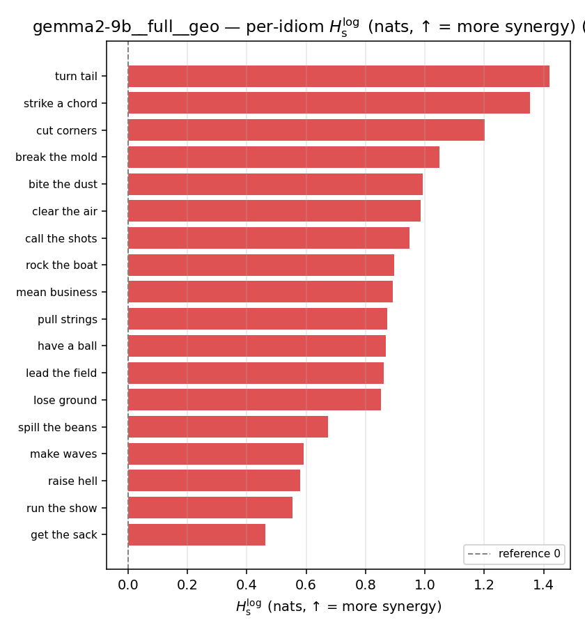 | 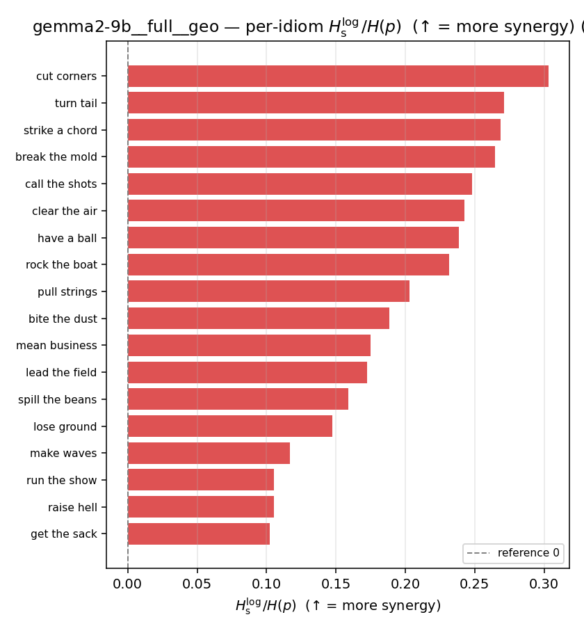 | 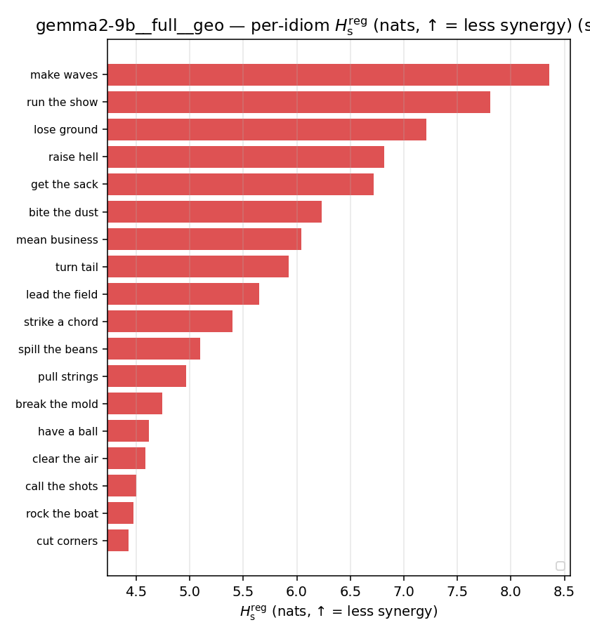 | 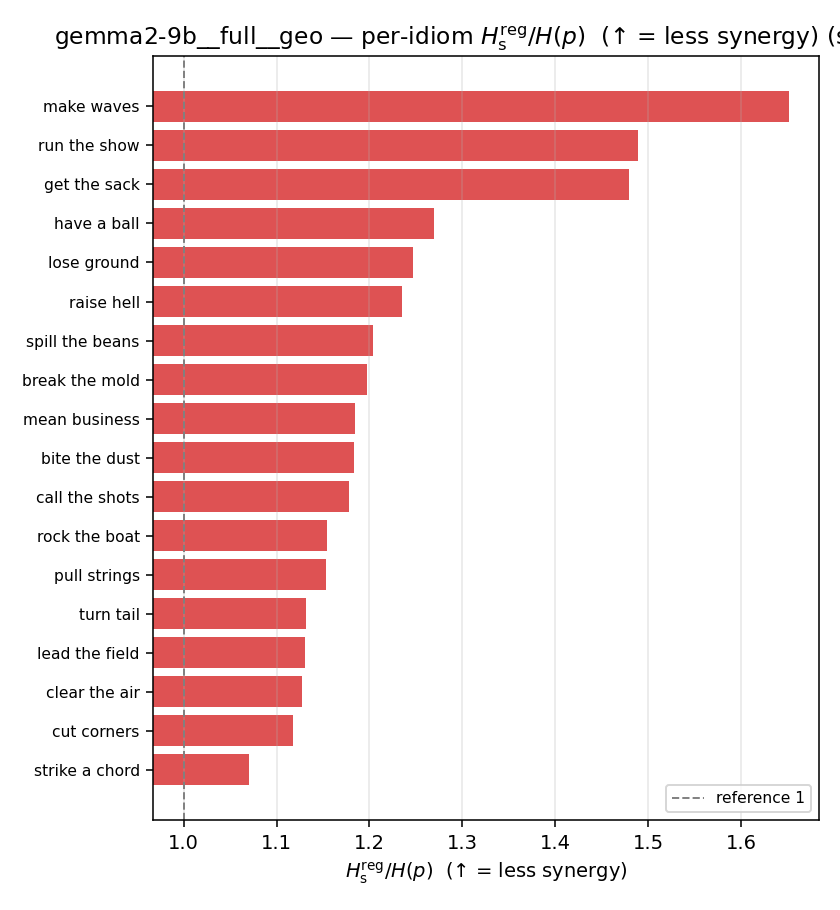 | 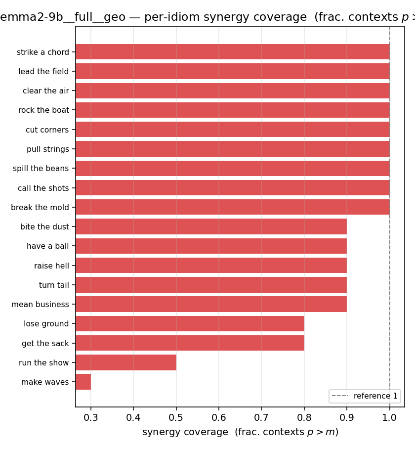 |
gemma2-9b · full · joint gemma2-9b__full__joint
| Ĥu/Ĥ ↑syn | Ĥu | Ĥs ↓syn | Ĥs/Ĥ ↓syn | Ĥslog ↑syn | Ĥslog/Ĥ ↑syn | Ĥsreg ↓syn | Ĥsreg/Ĥ ↓syn | f̂syn ↑syn | |
|---|---|---|---|---|---|---|---|---|---|
| strip (per-phrase) | 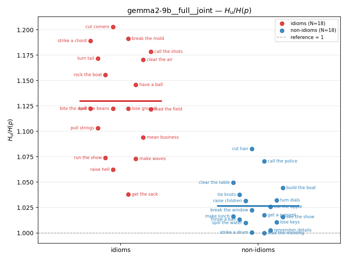 | 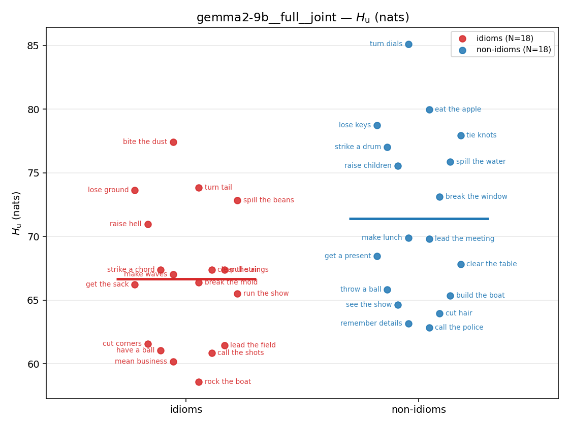 | 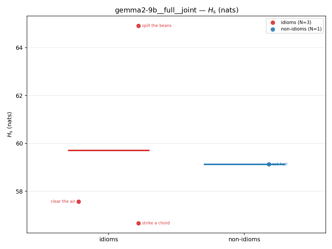 | 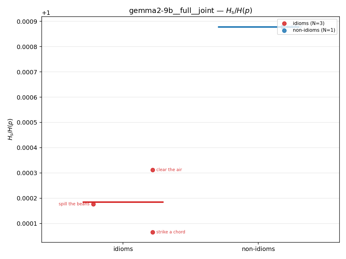 | 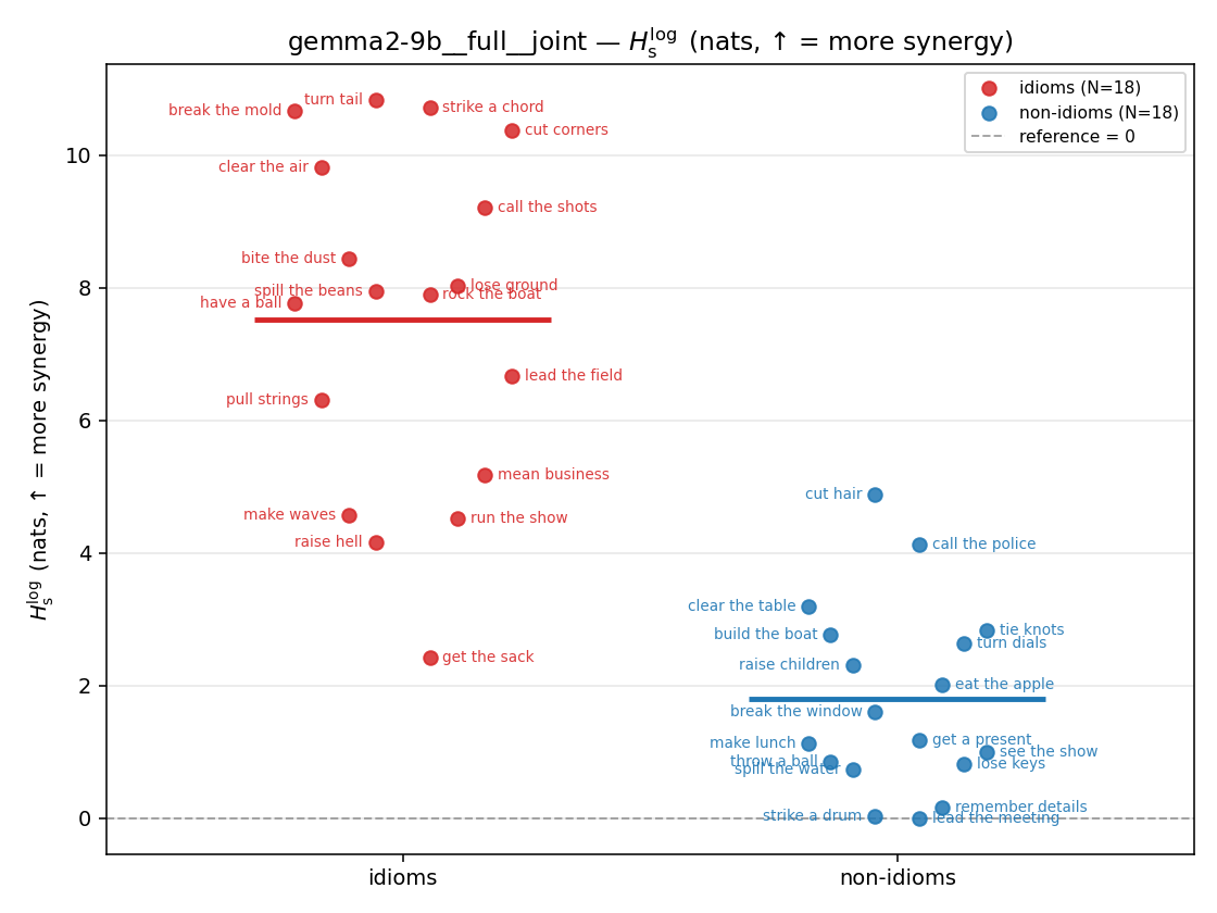 | 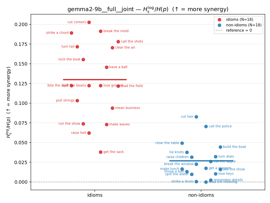 | 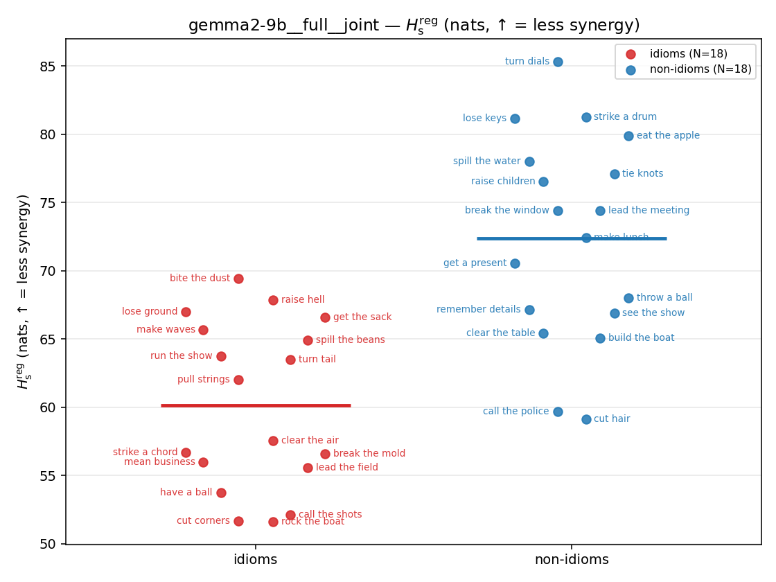 | 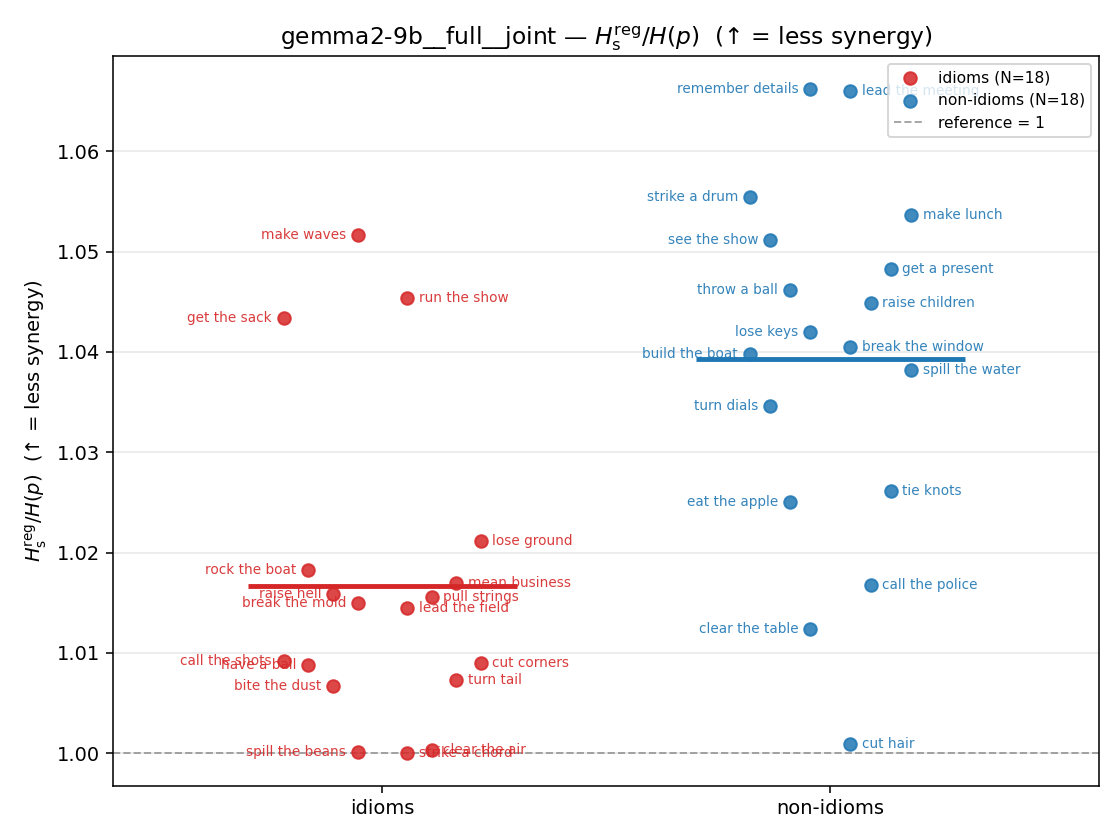 | 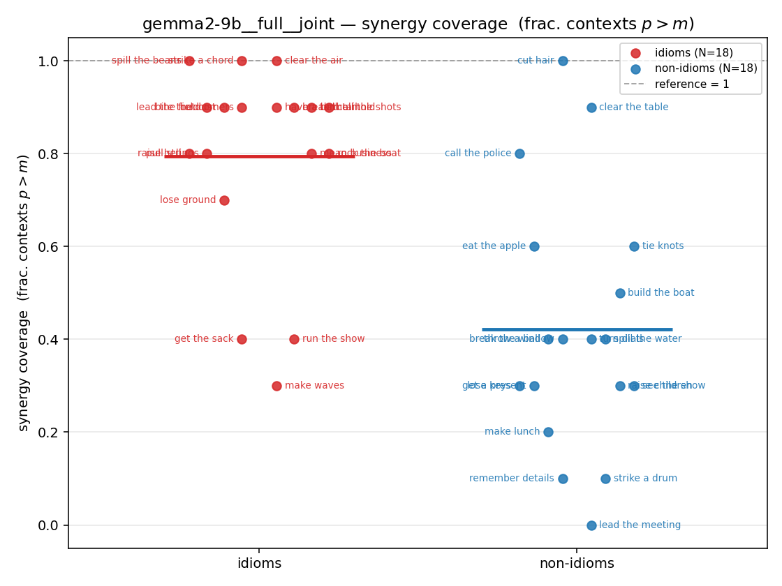 |
| mean ± 95% CI | 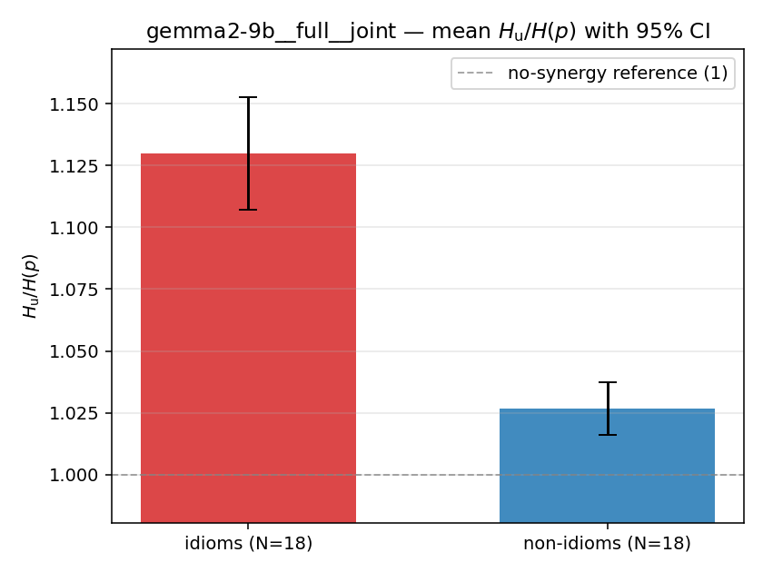 | 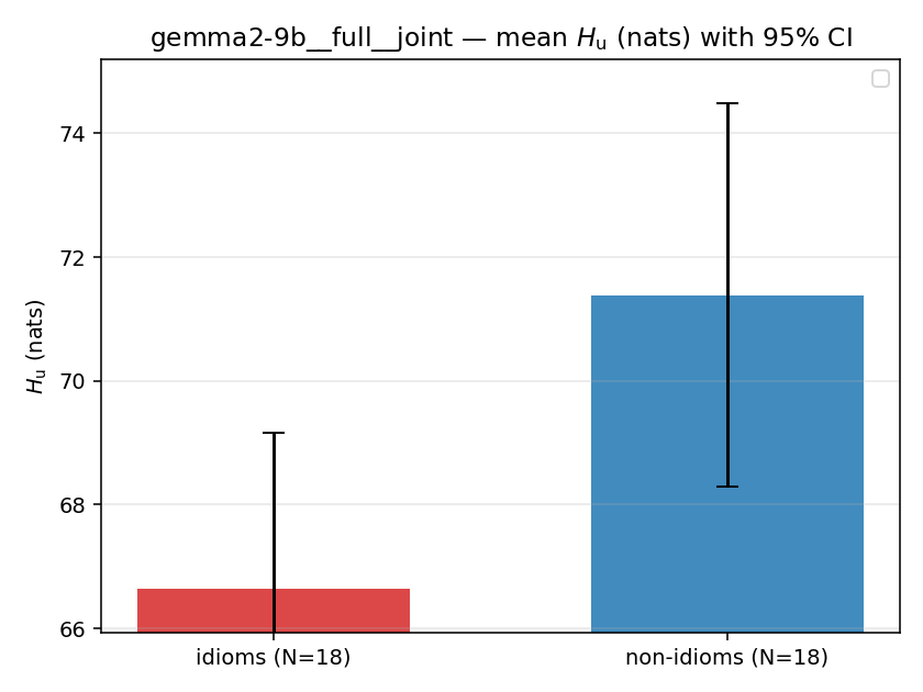 | 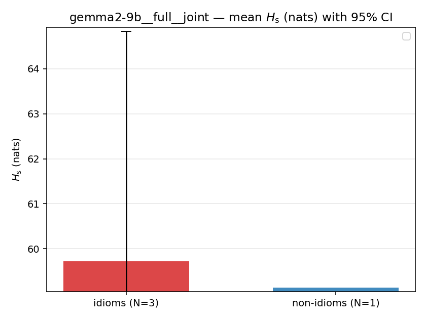 | 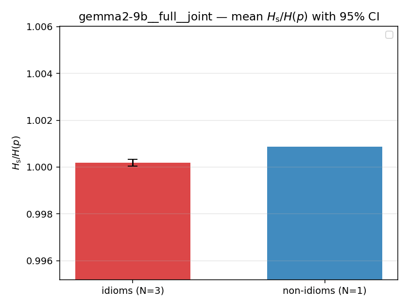 | 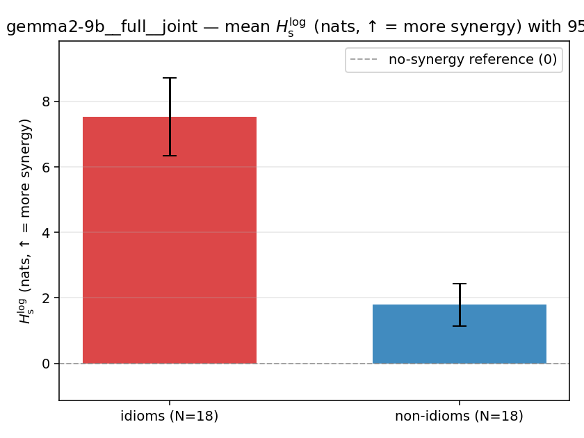 | 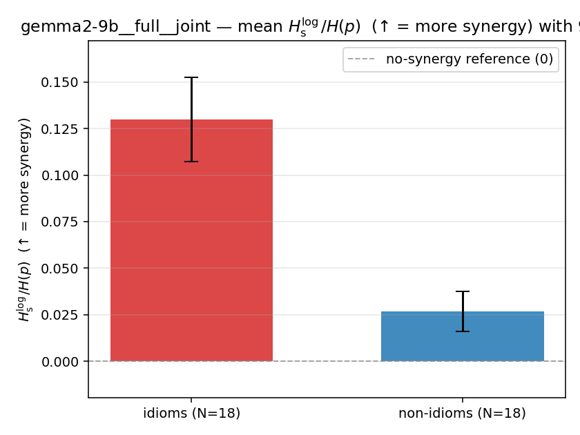 | 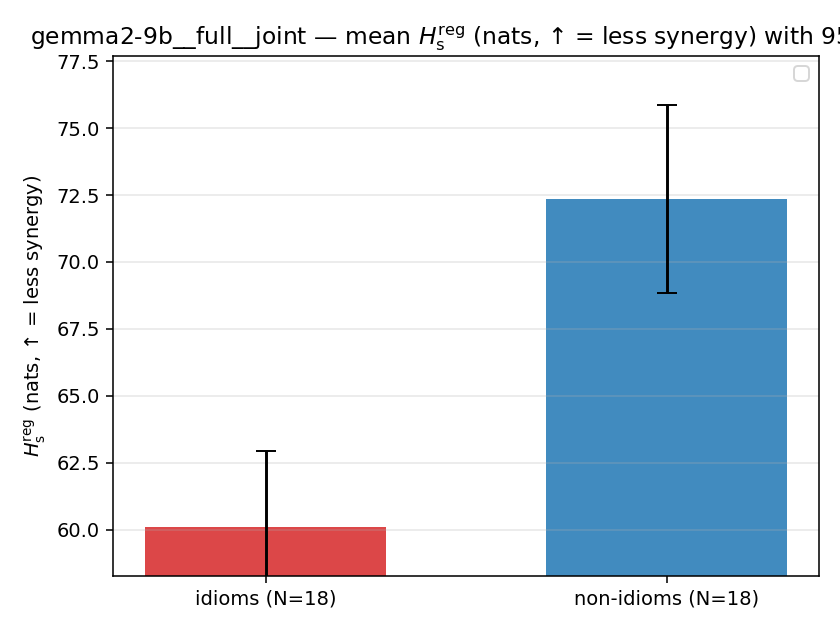 | 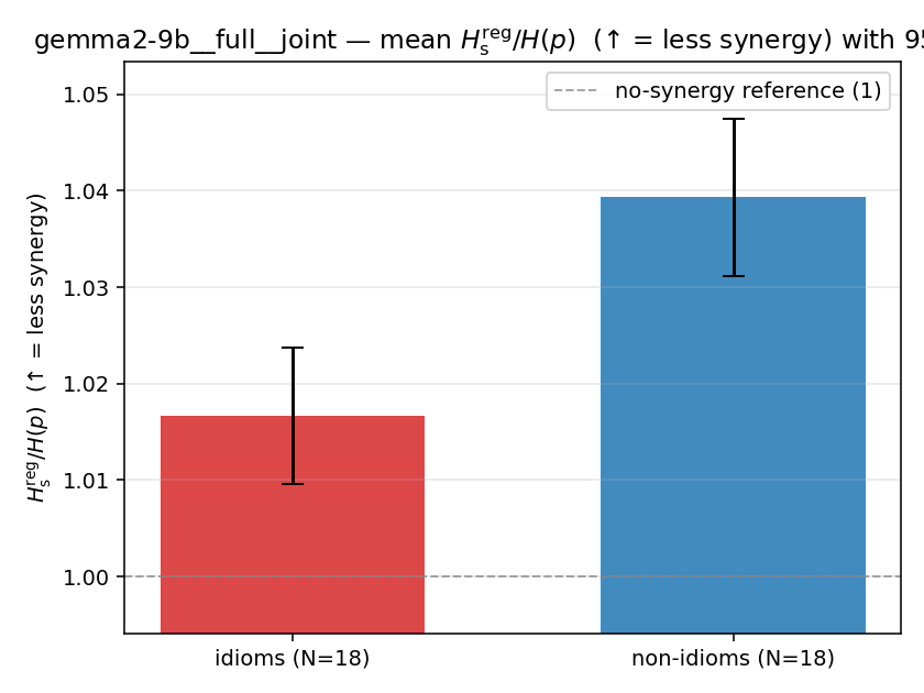 | 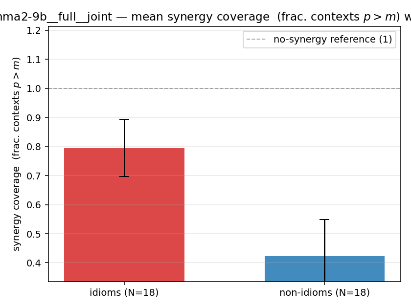 |
| per-idiom (sorted) | 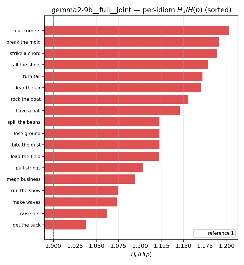 | 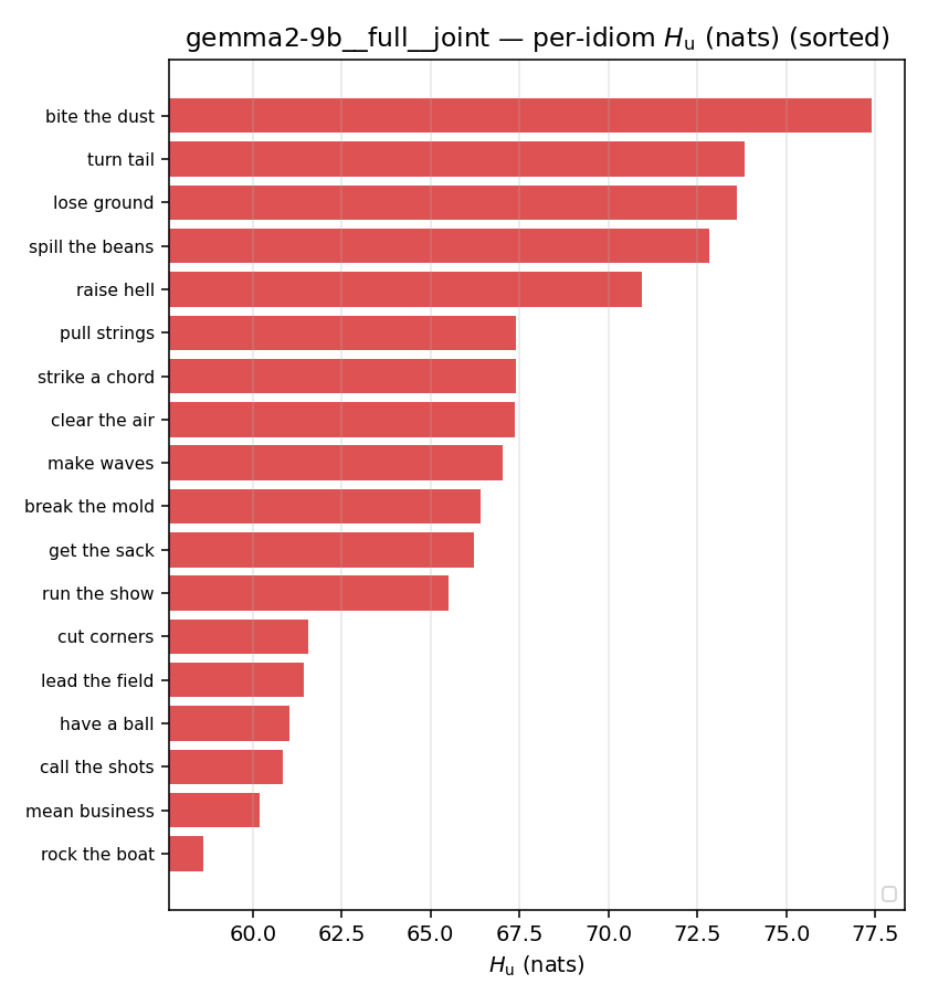 | 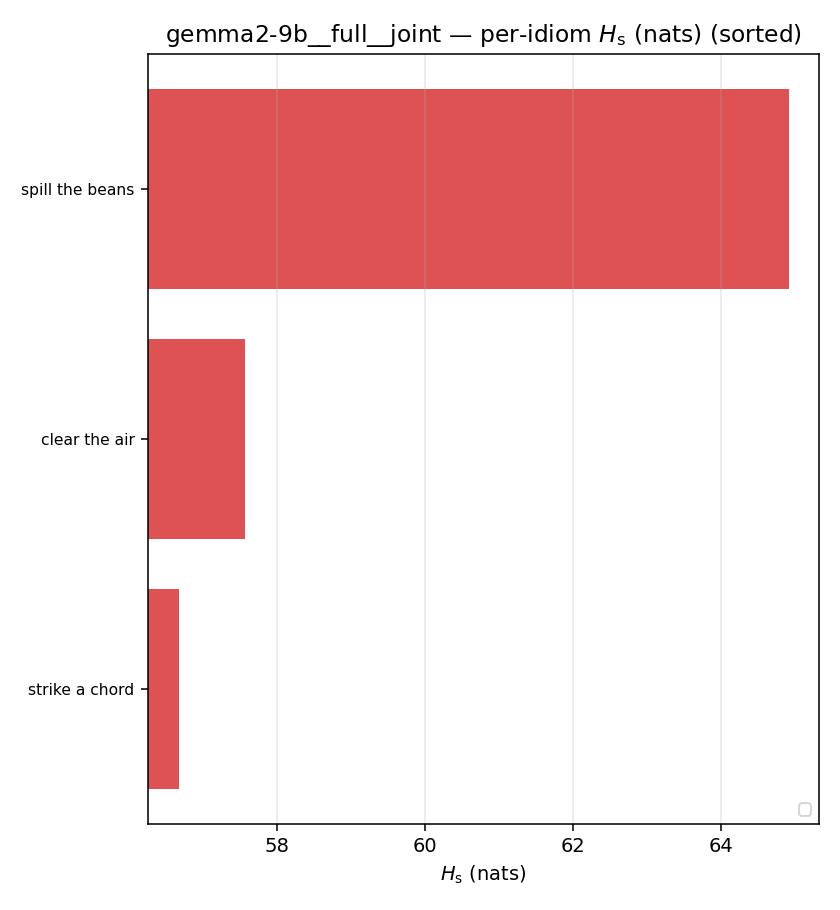 | 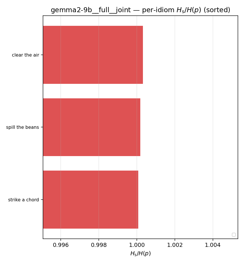 | 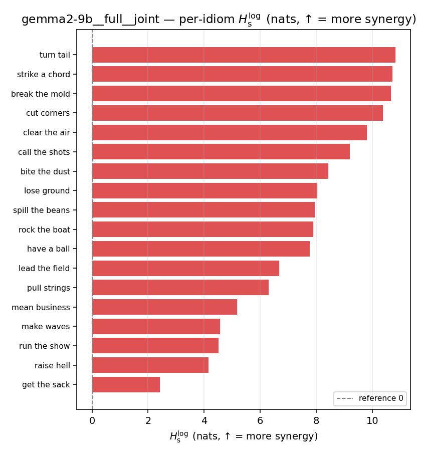 | 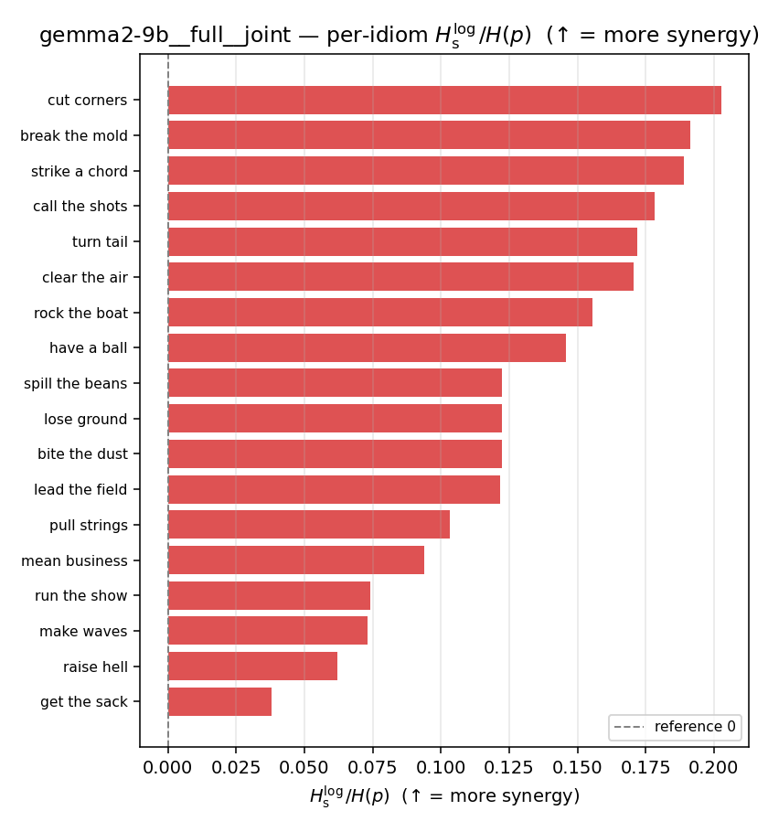 | 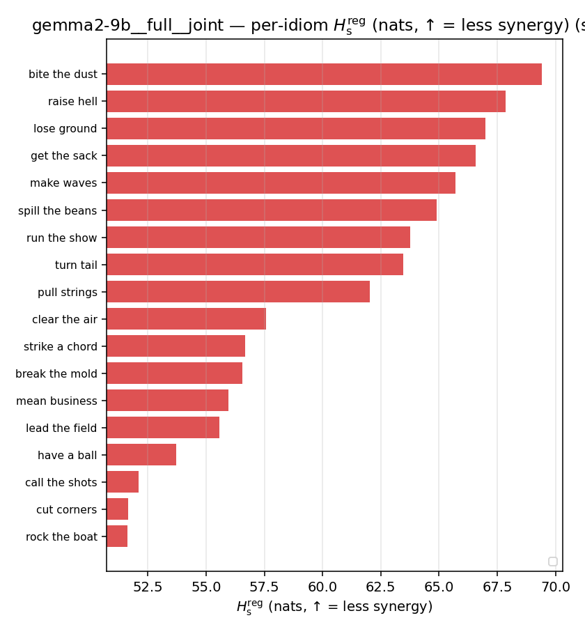 | 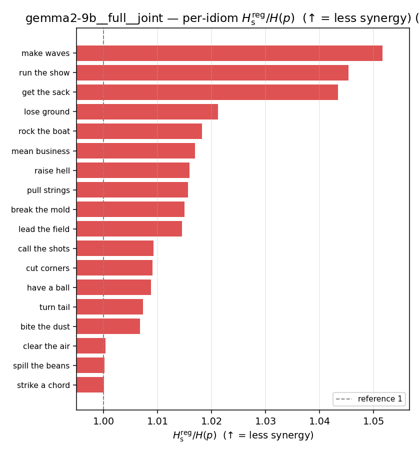 | 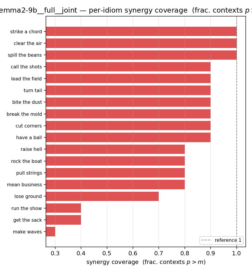 |
qwen3-8b-base — per-config figures
3×9 grid of figure-type × metric (↑syn / ↓syn in a header = the metric increases / decreases with synergy; definitions on the entropies page). Tables scroll horizontally; “— (no finite values)” marks Ĥs/ratio_s panels where every phrase was +inf. Click to zoom.
qwen3-8b-base · medial · geo qwen3-8b-base__medial__geo
| Ĥu/Ĥ ↑syn | Ĥu | Ĥs ↓syn | Ĥs/Ĥ ↓syn | Ĥslog ↑syn | Ĥslog/Ĥ ↑syn | Ĥsreg ↓syn | Ĥsreg/Ĥ ↓syn | f̂syn ↑syn | |
|---|---|---|---|---|---|---|---|---|---|
| strip (per-phrase) | 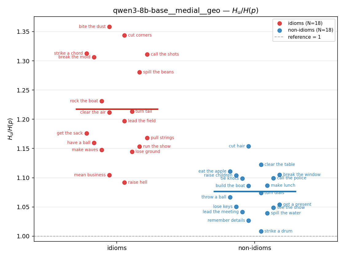 | 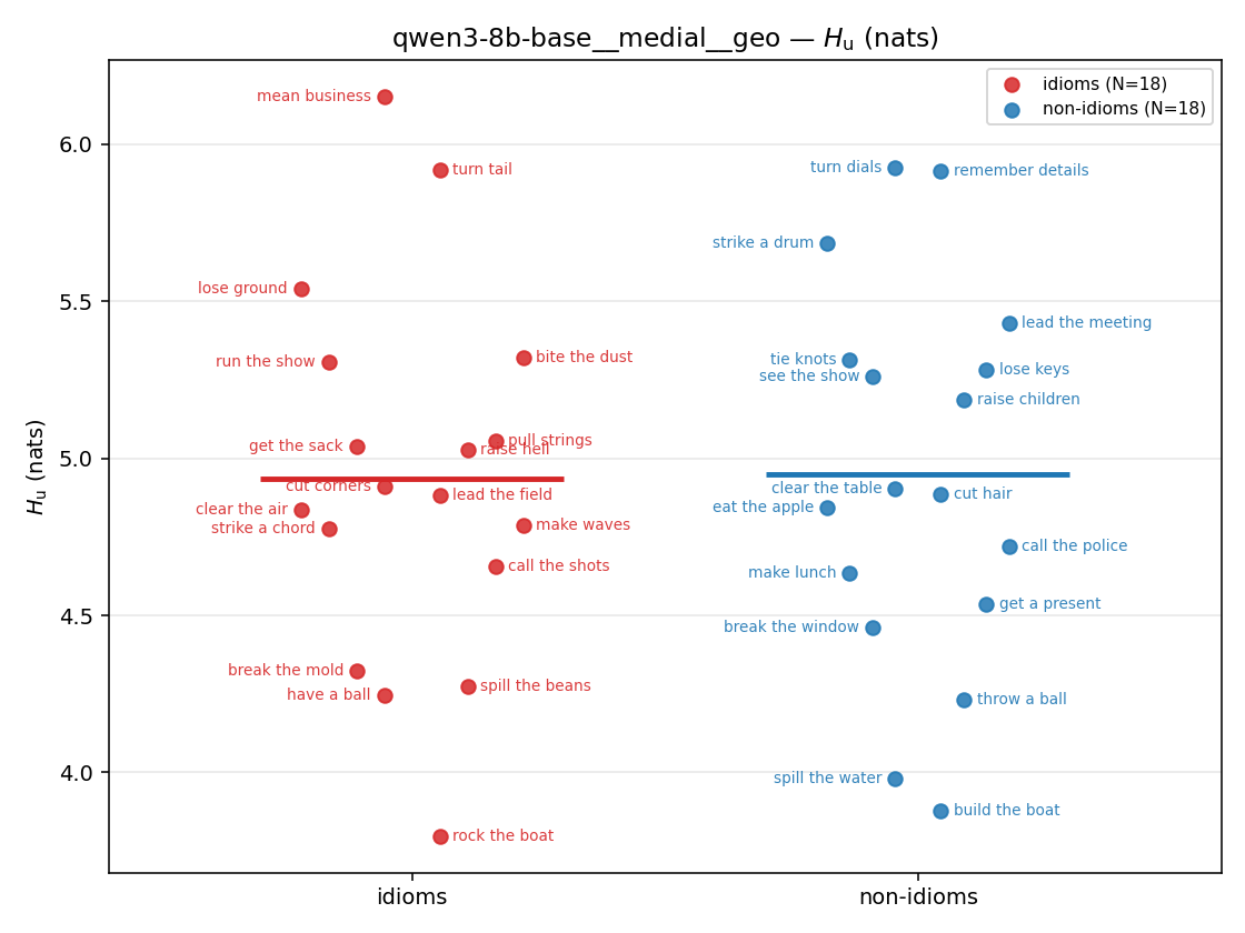 | 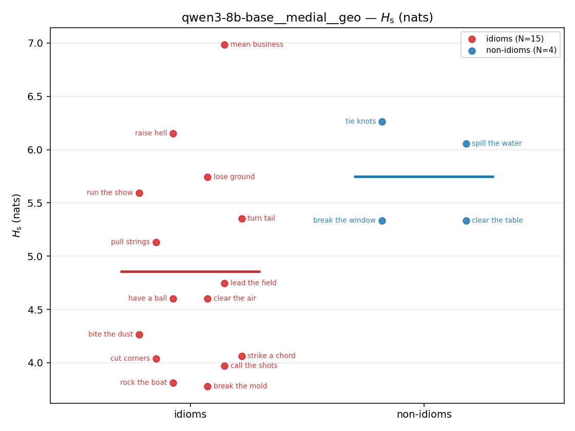 | 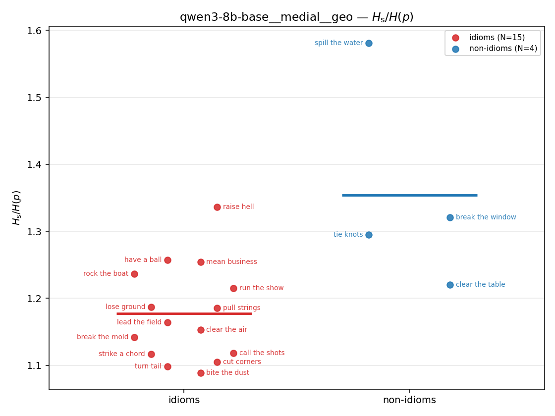 | 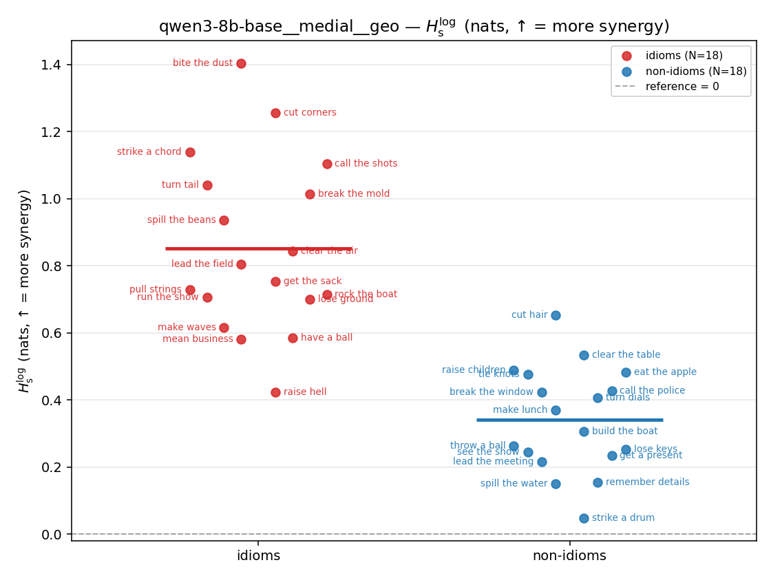 | 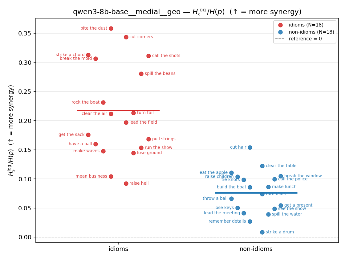 | 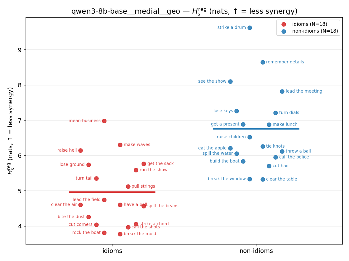 | 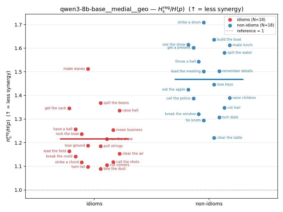 | 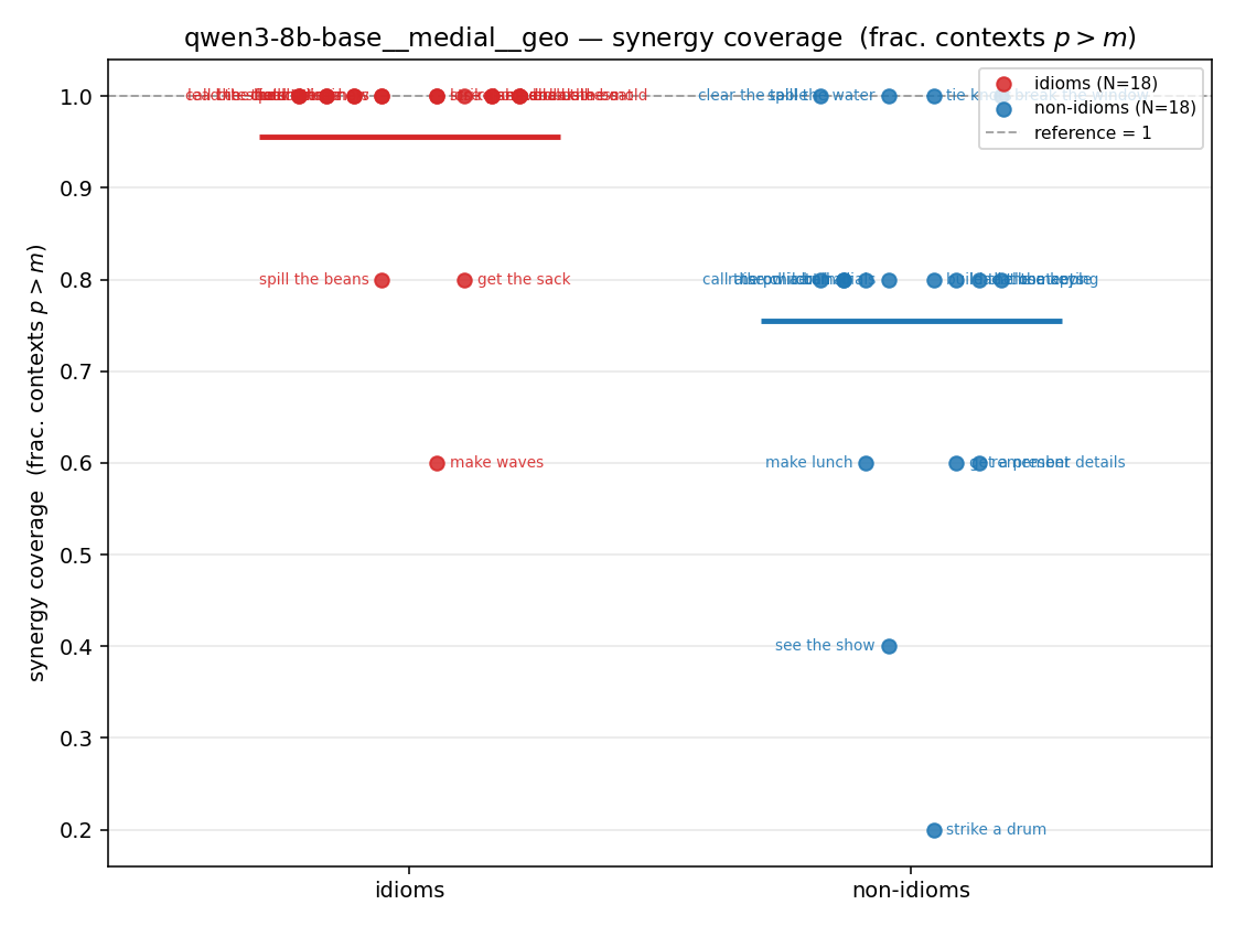 |
| mean ± 95% CI | 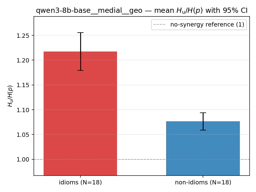 | 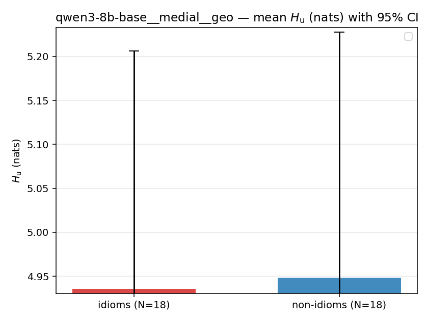 | 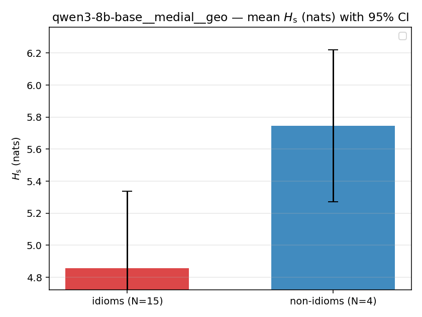 | 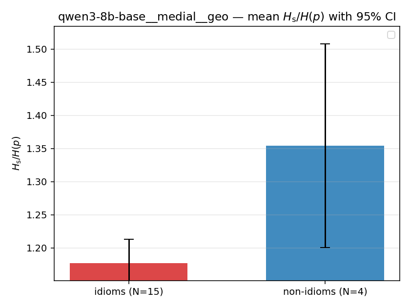 | 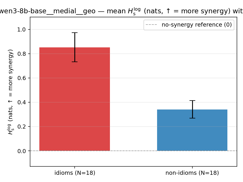 | 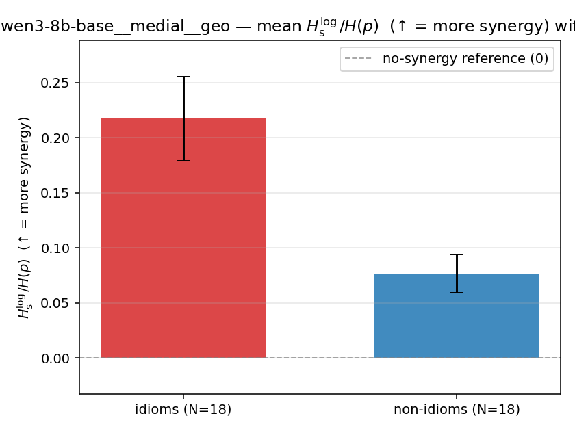 | 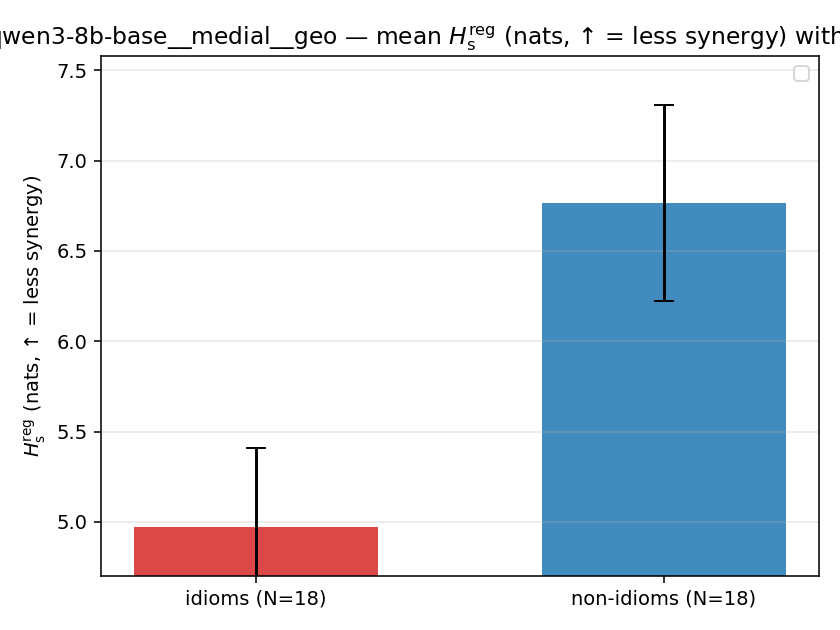 | 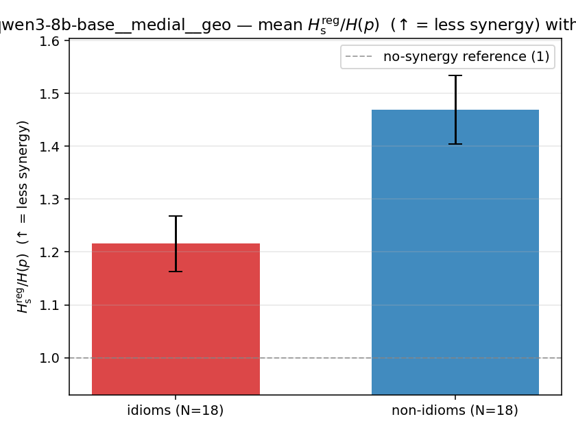 | 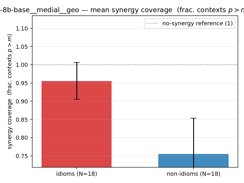 |
| per-idiom (sorted) | 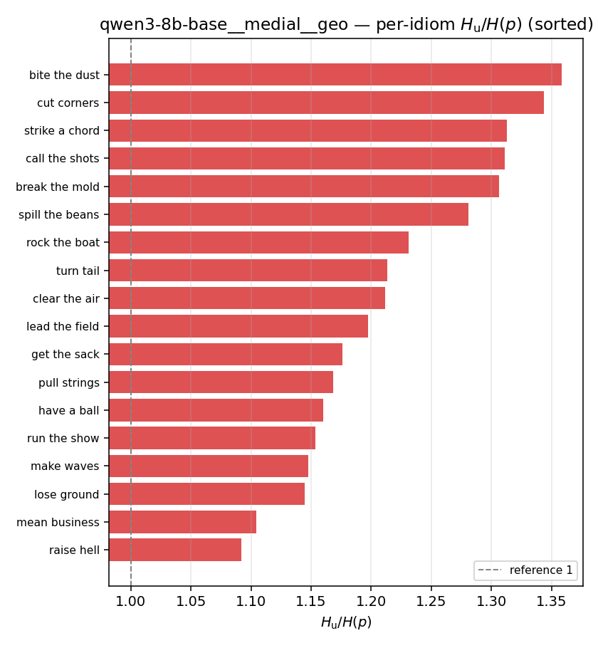 | 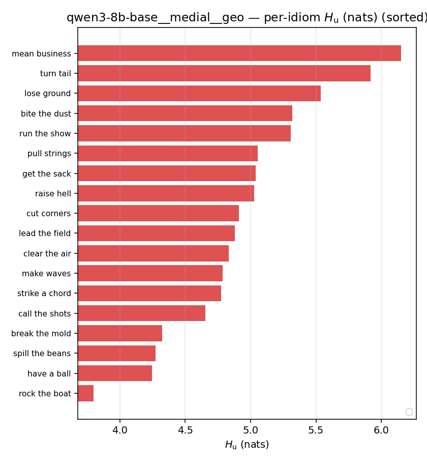 | 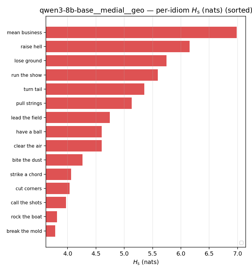 | 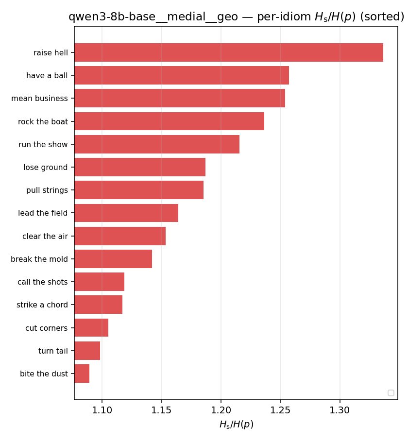 | 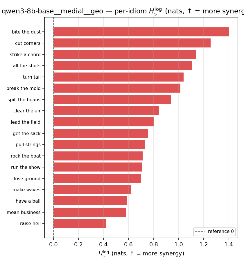 | 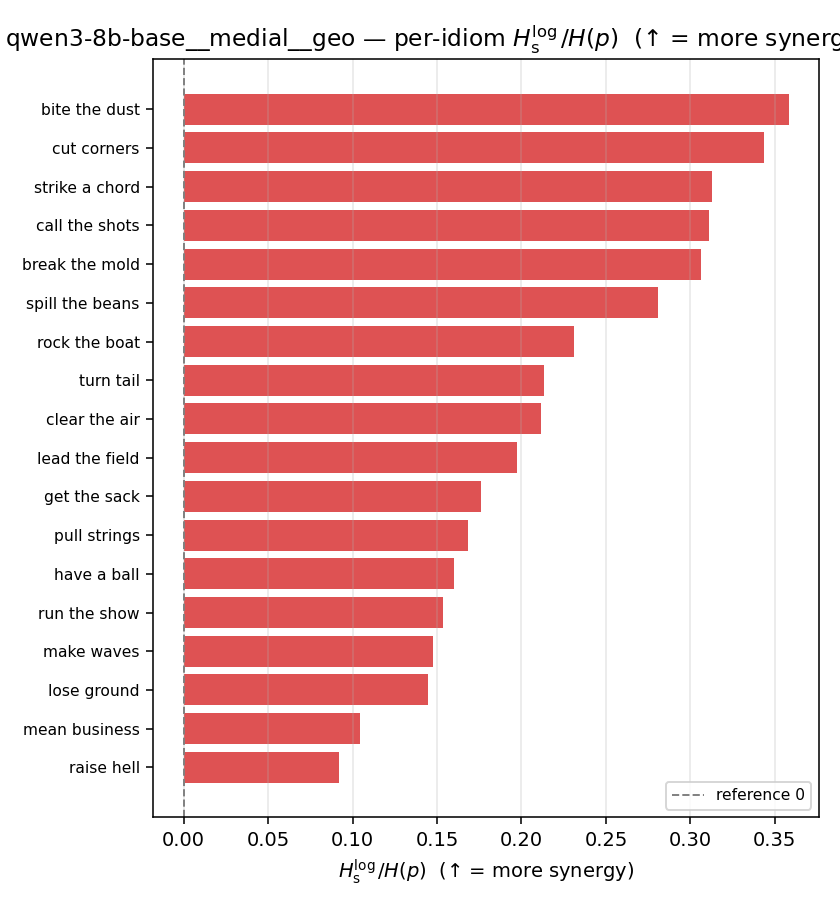 | 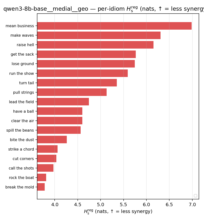 | 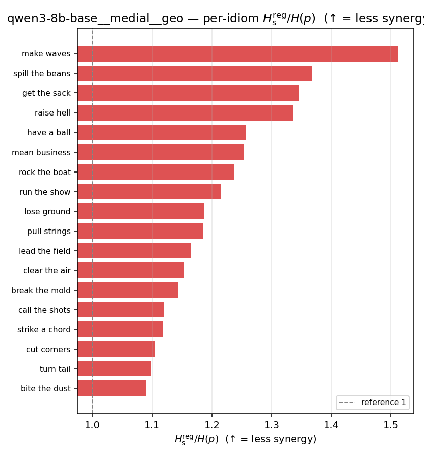 | 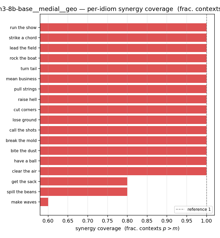 |
qwen3-8b-base · medial · joint qwen3-8b-base__medial__joint
| Ĥu/Ĥ ↑syn | Ĥu | Ĥs ↓syn | Ĥs/Ĥ ↓syn | Ĥslog ↑syn | Ĥslog/Ĥ ↑syn | Ĥsreg ↓syn | Ĥsreg/Ĥ ↓syn | f̂syn ↑syn | |
|---|---|---|---|---|---|---|---|---|---|
| strip (per-phrase) | 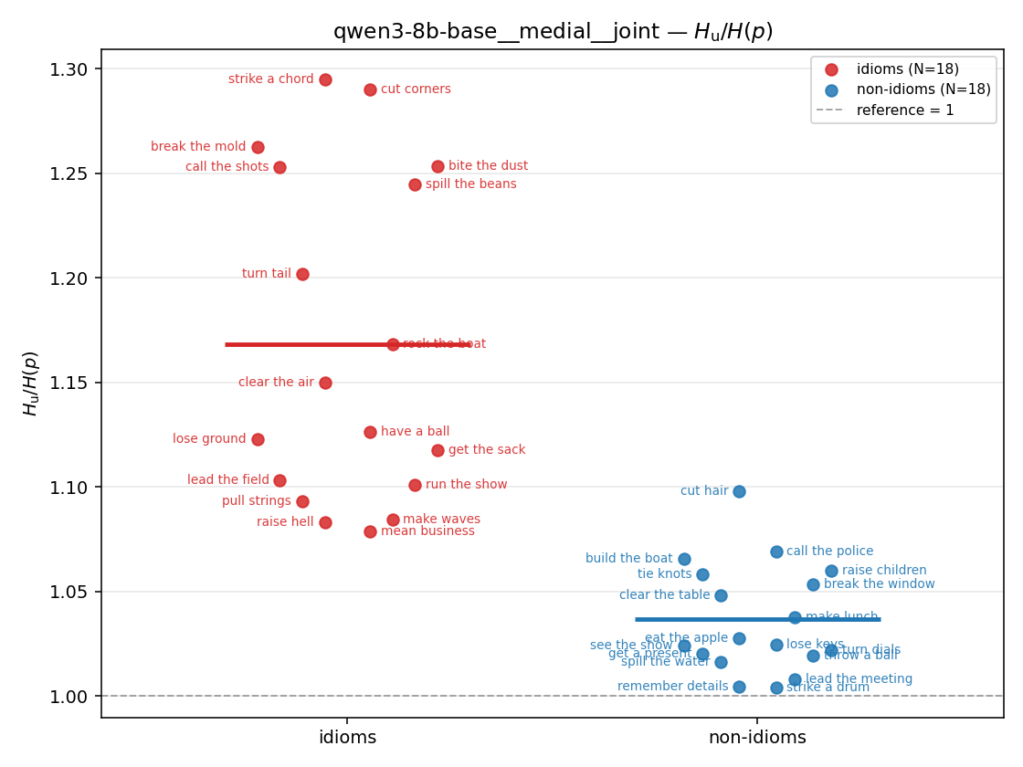 | 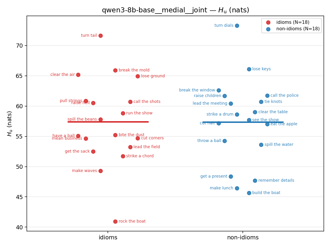 | — (no finite values) | — (no finite values) | 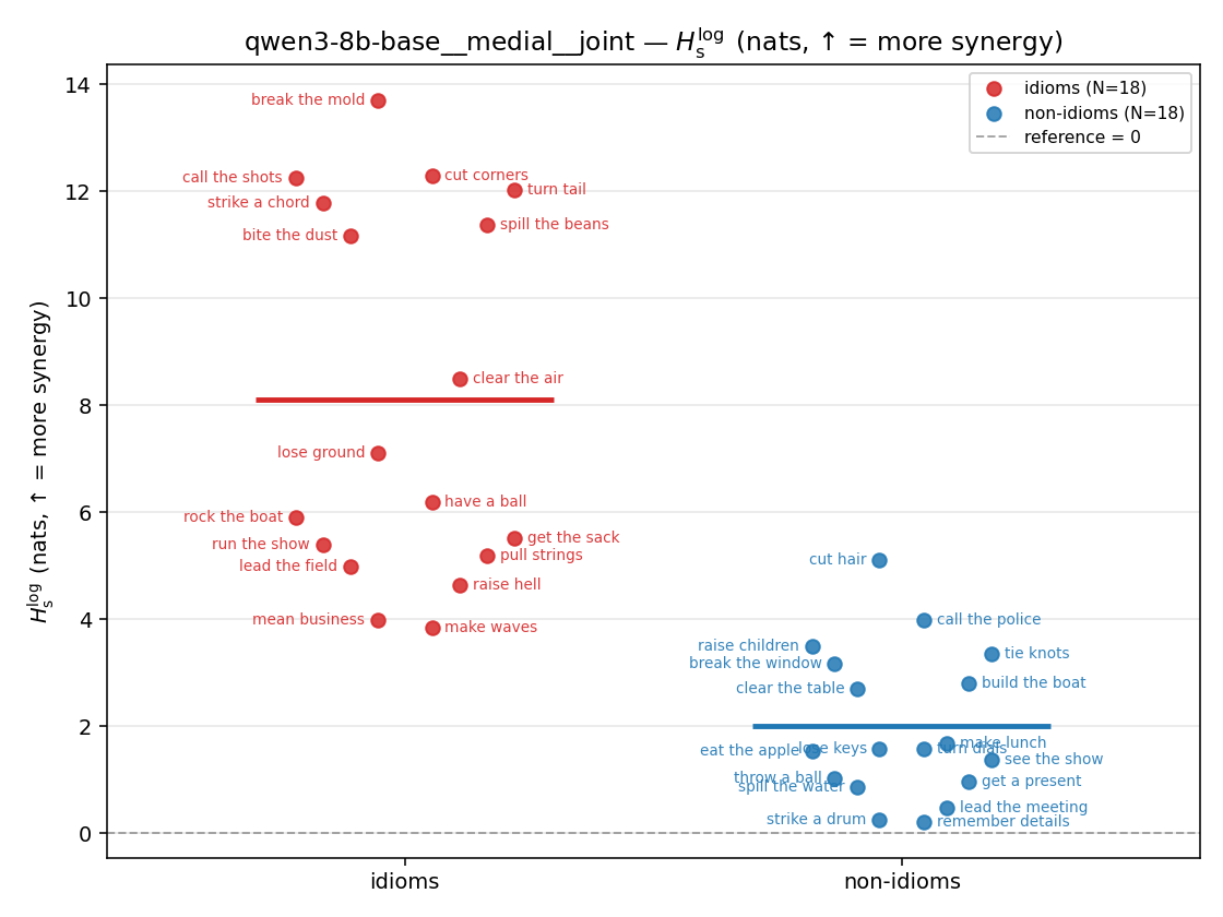 | 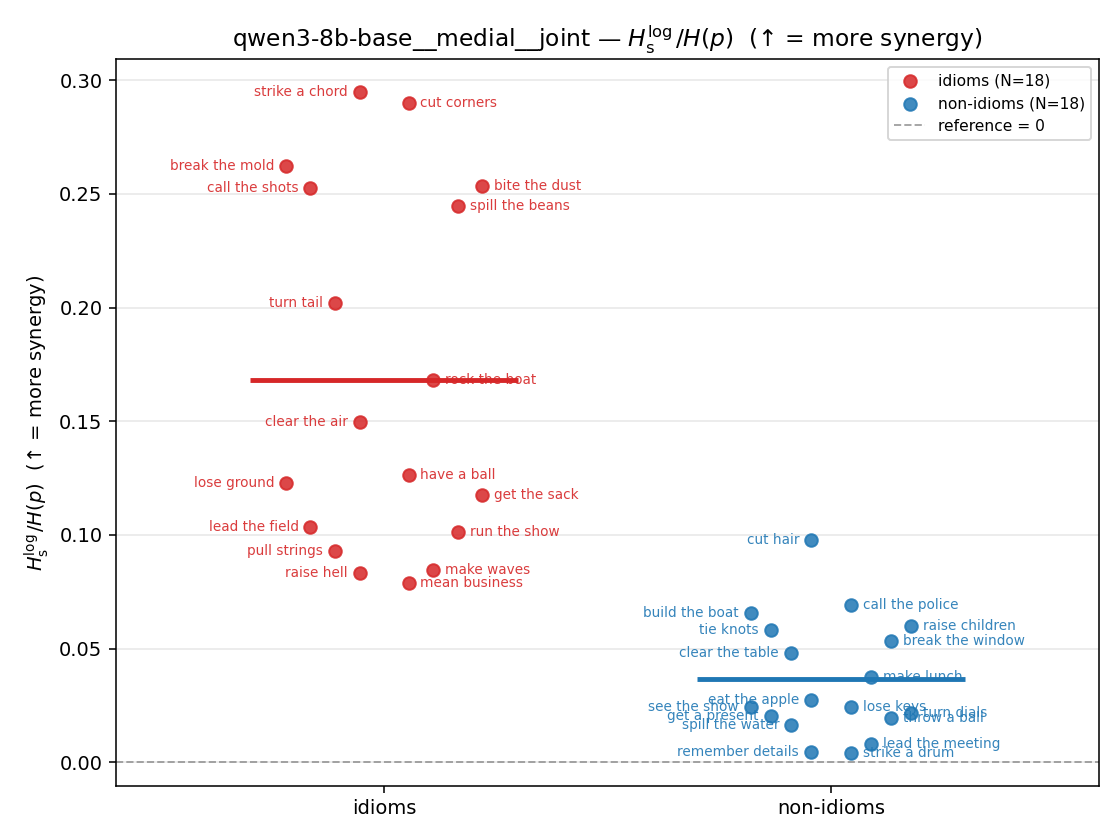 | 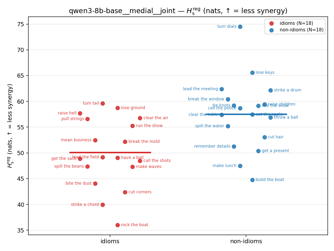 | 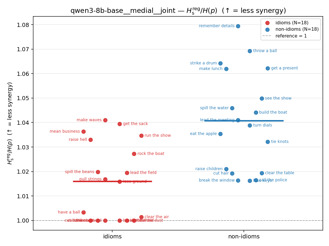 | 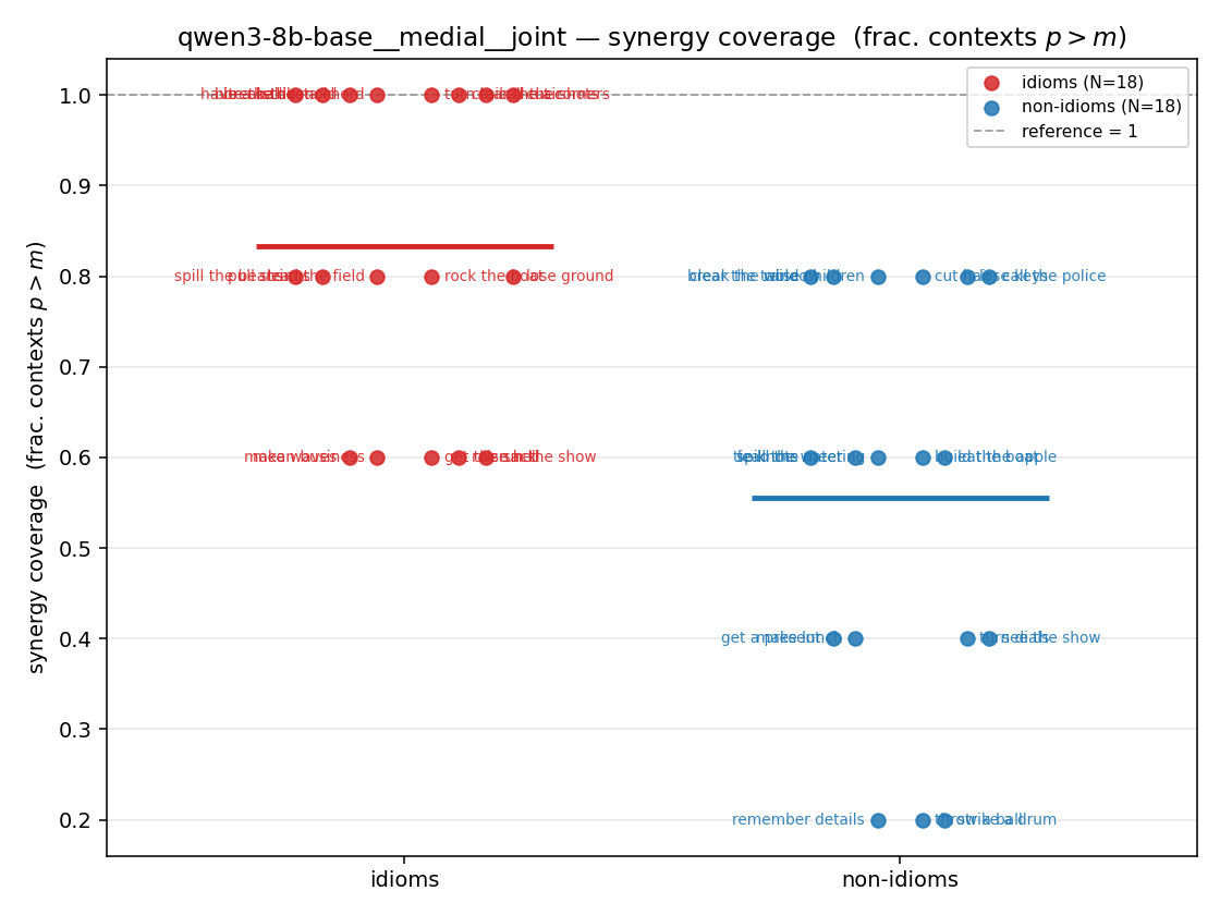 |
| mean ± 95% CI | 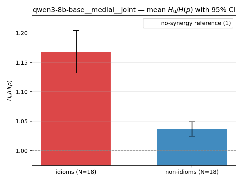 | 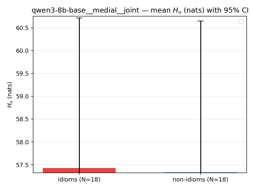 | — (no finite values) | — (no finite values) | 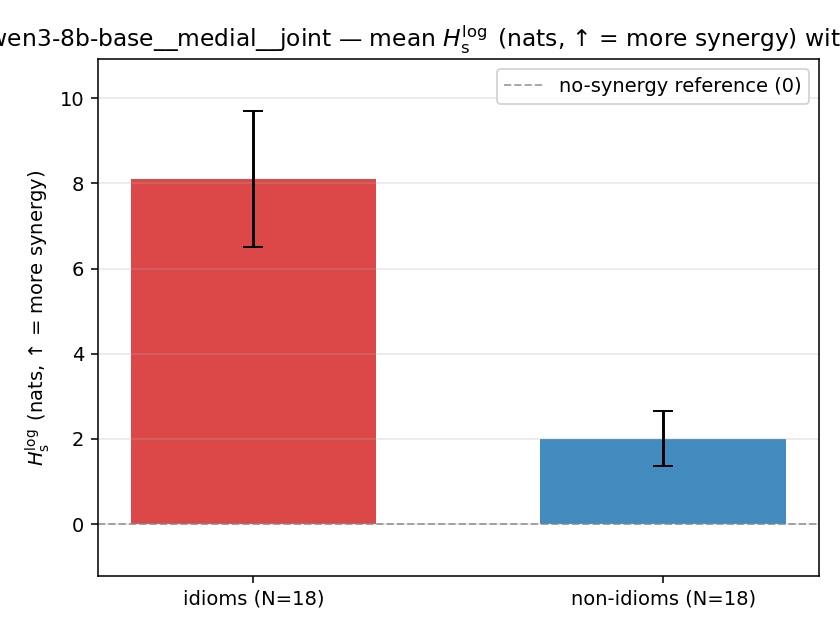 | 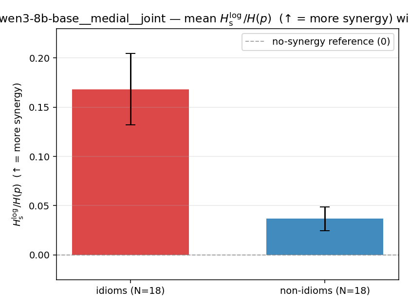 | 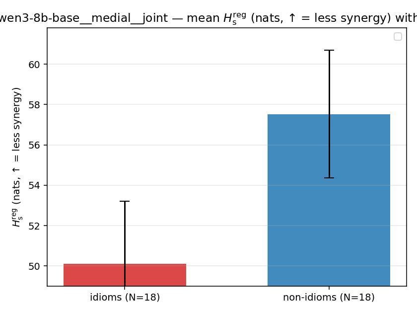 | 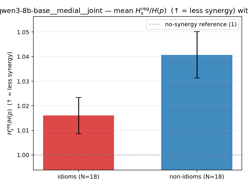 | 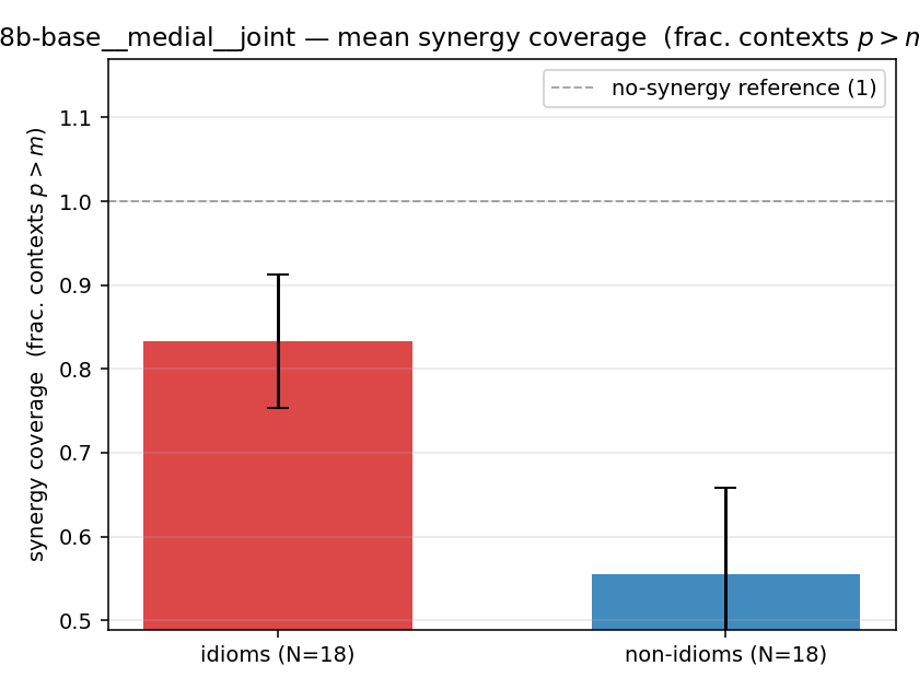 |
| per-idiom (sorted) | 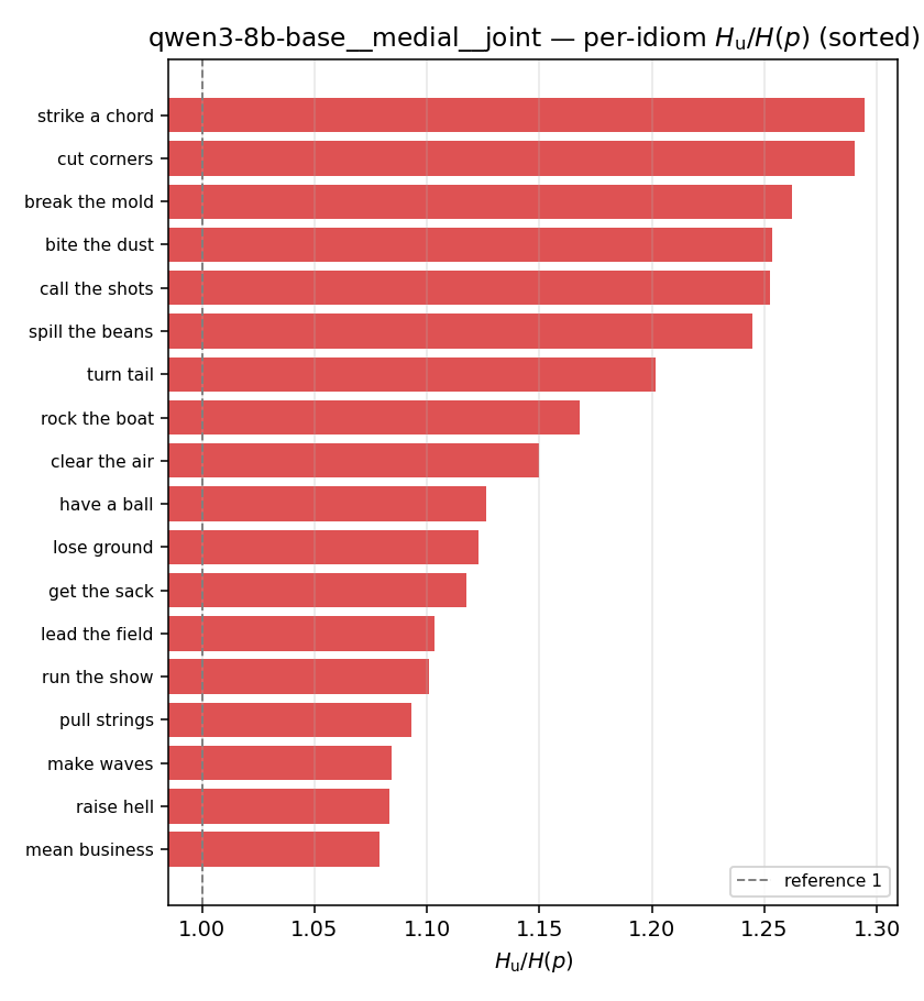 | 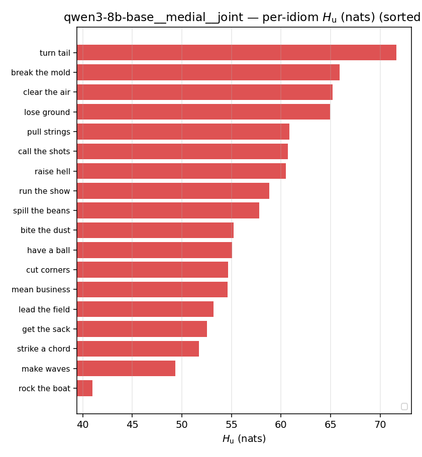 | — (no finite values) | — (no finite values) | 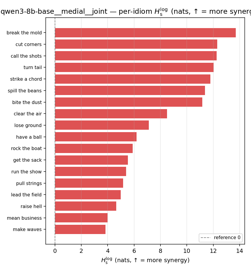 | 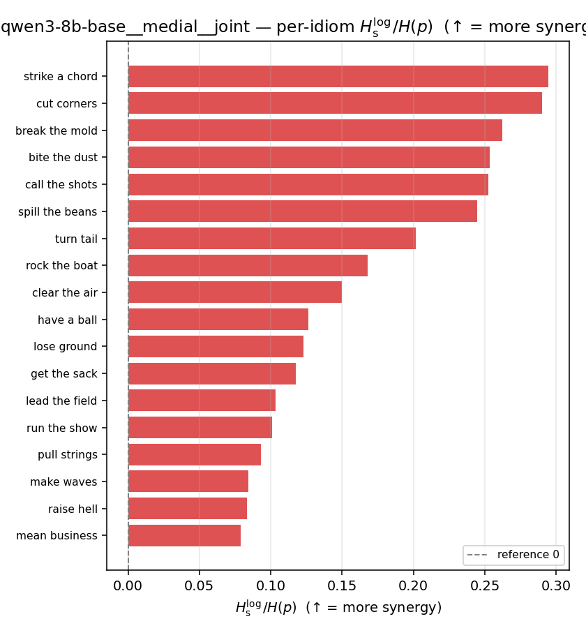 | 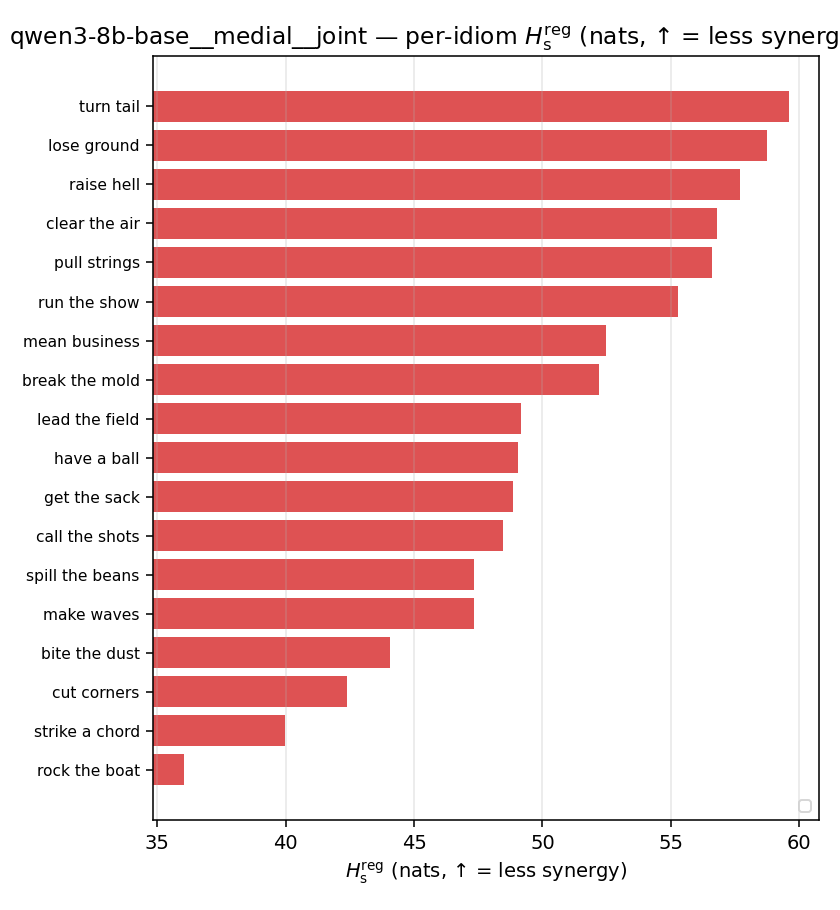 | 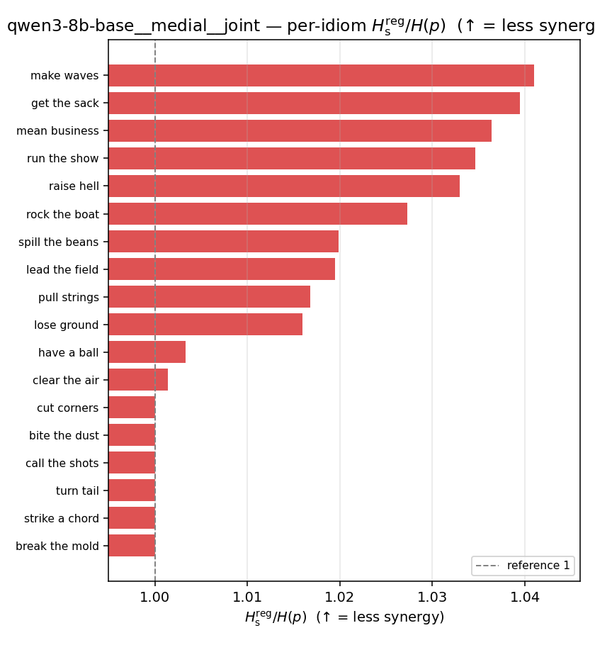 | 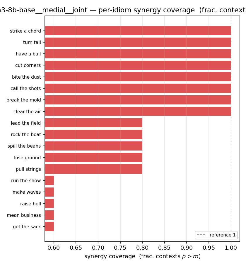 |
qwen3-8b-base · full · geo qwen3-8b-base__full__geo
| Ĥu/Ĥ ↑syn | Ĥu | Ĥs ↓syn | Ĥs/Ĥ ↓syn | Ĥslog ↑syn | Ĥslog/Ĥ ↑syn | Ĥsreg ↓syn | Ĥsreg/Ĥ ↓syn | f̂syn ↑syn | |
|---|---|---|---|---|---|---|---|---|---|
| strip (per-phrase) | 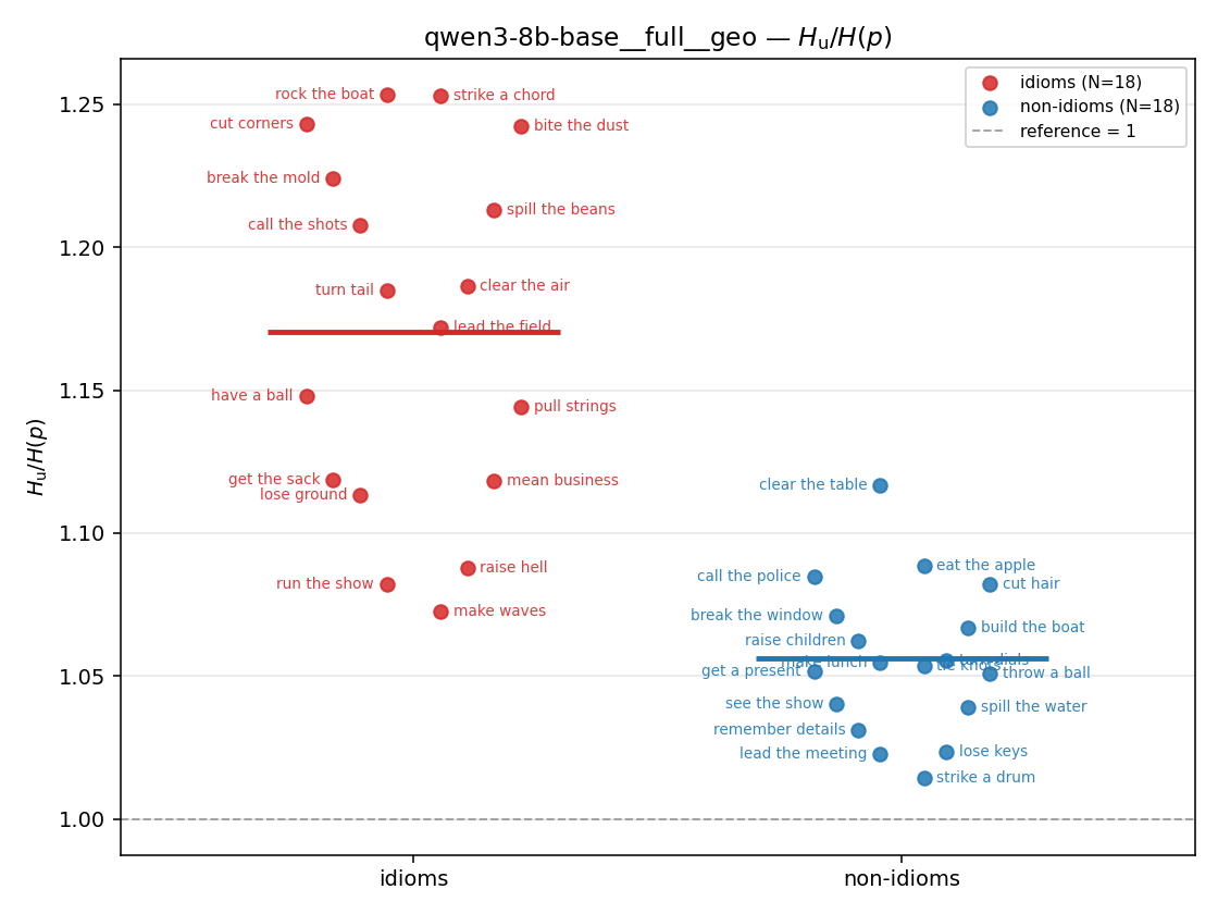 | 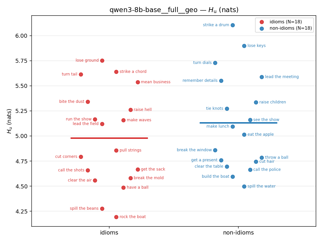 | — (no finite values) | — (no finite values) | 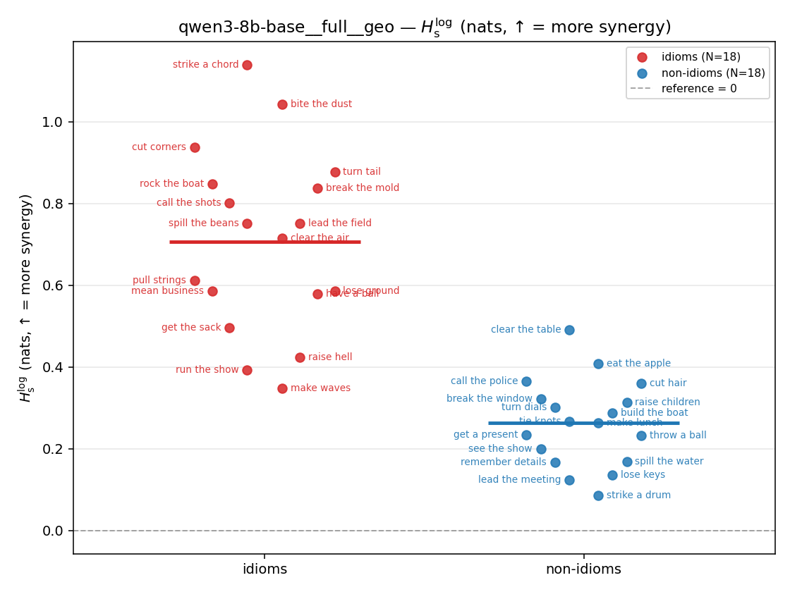 | 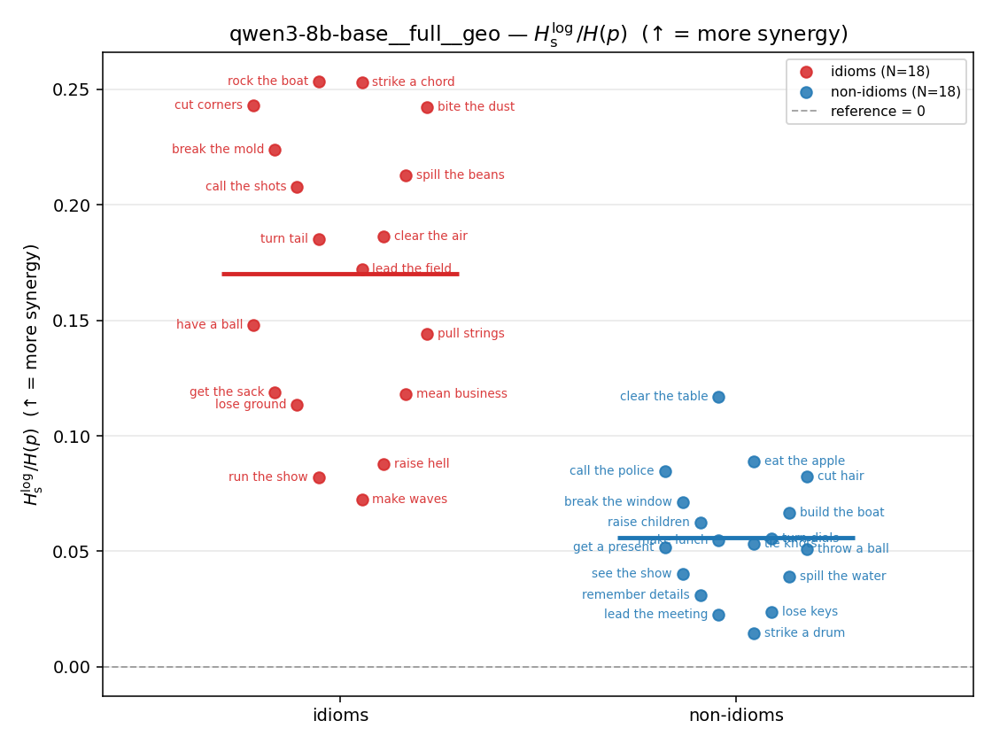 | 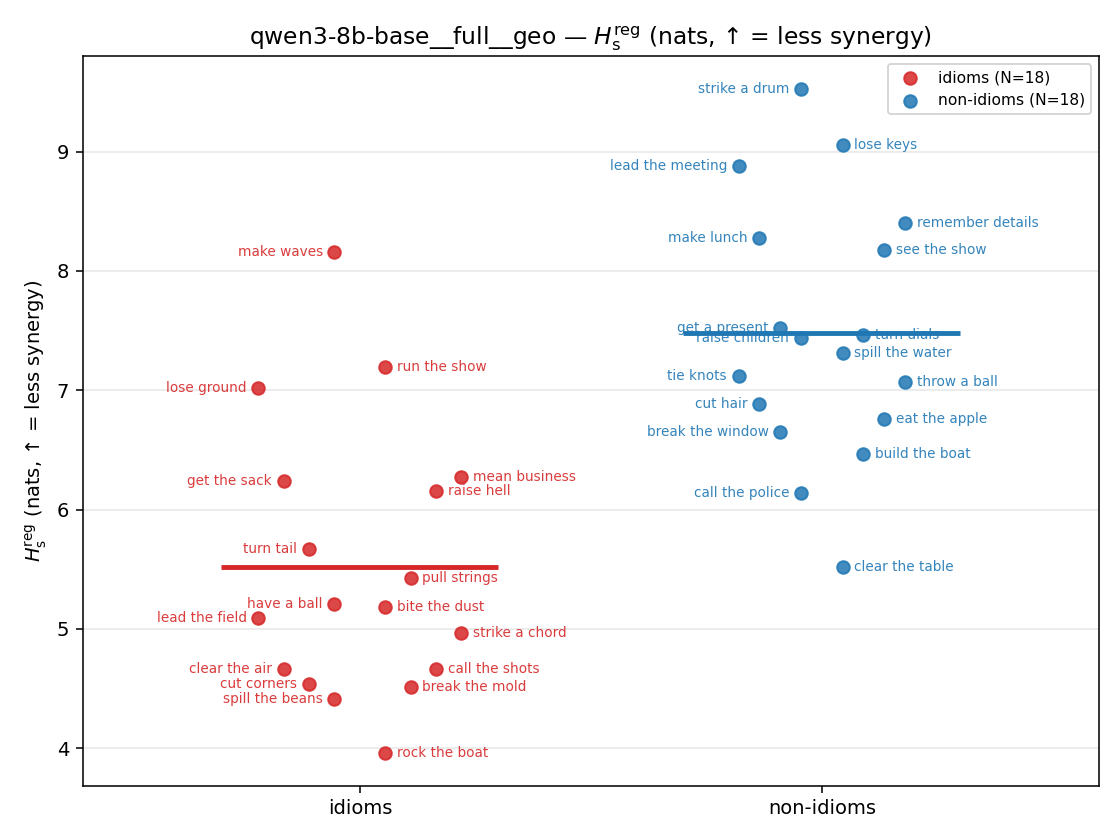 | 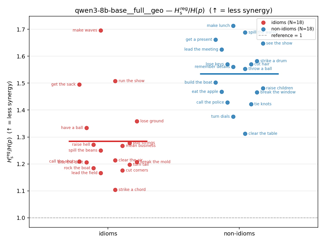 | 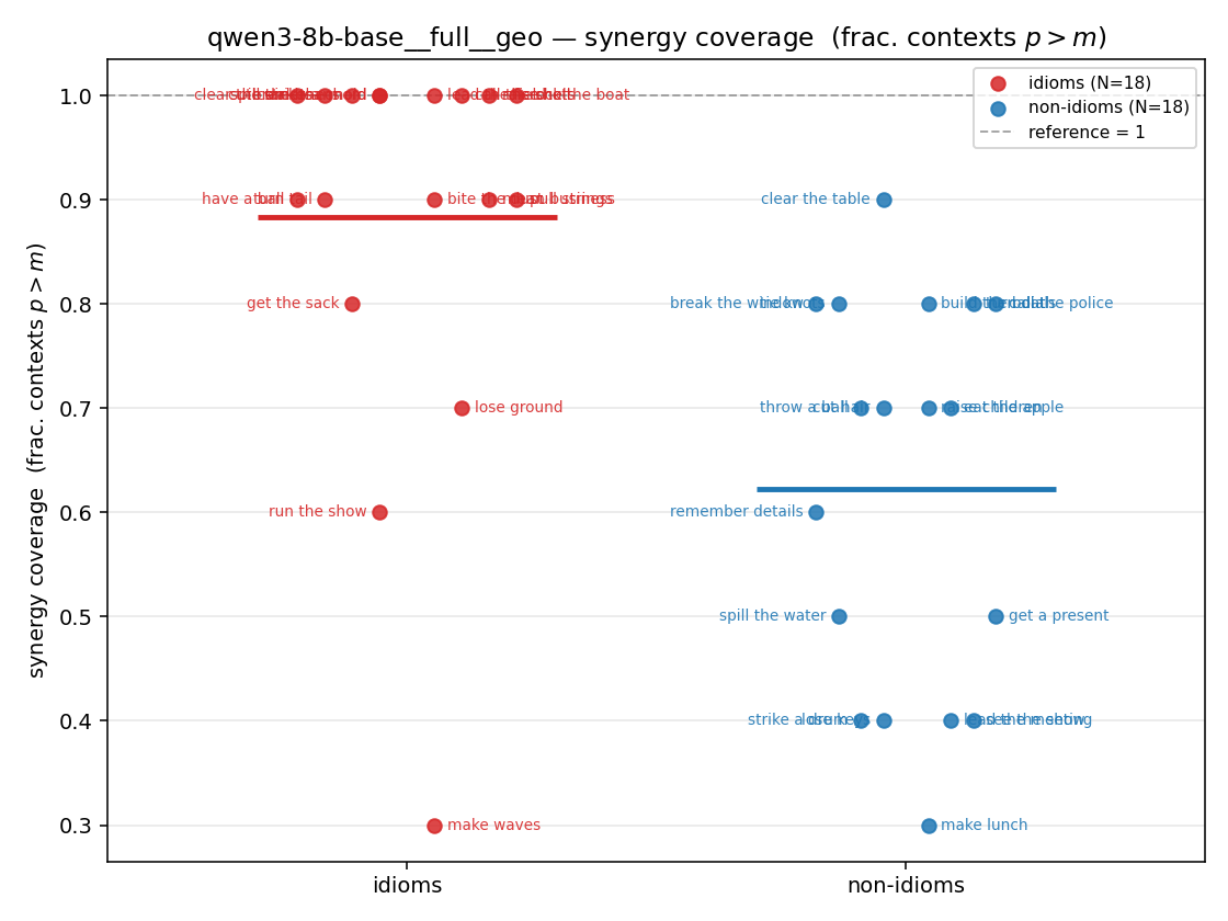 |
| mean ± 95% CI | 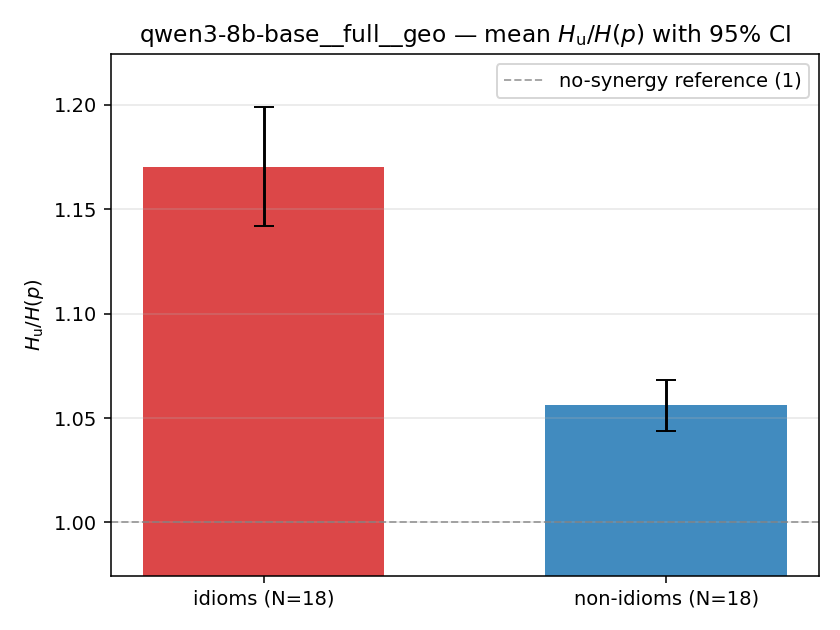 | 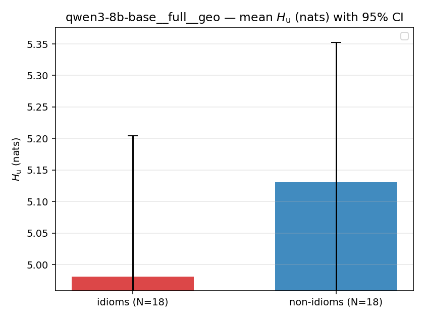 | — (no finite values) | — (no finite values) | 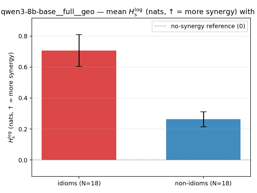 | 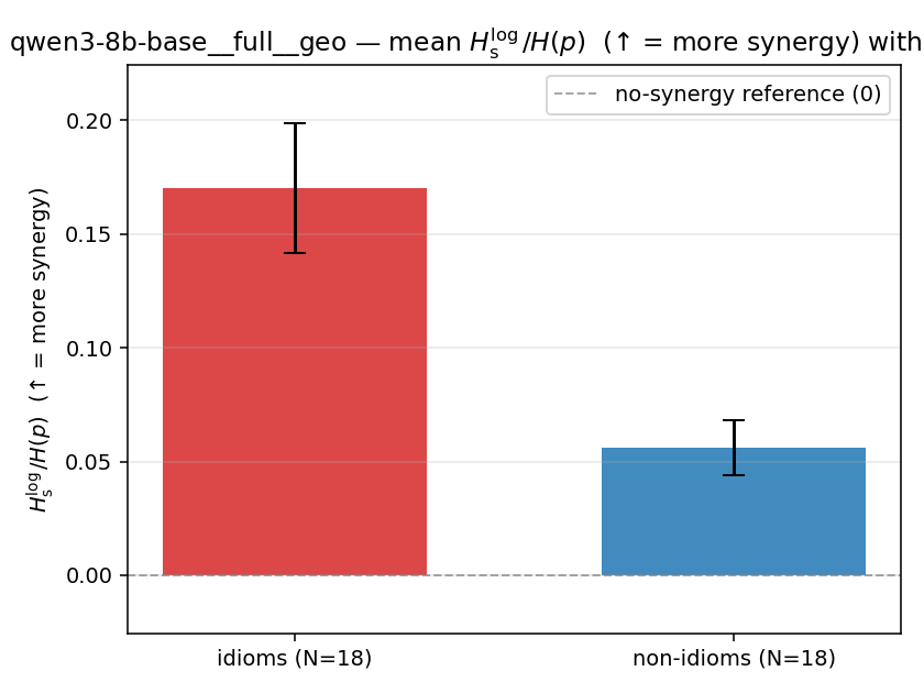 | 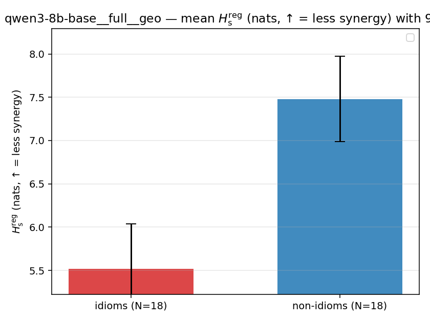 | 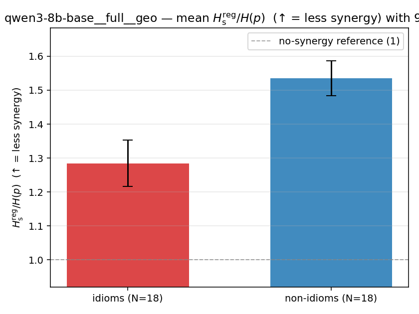 | 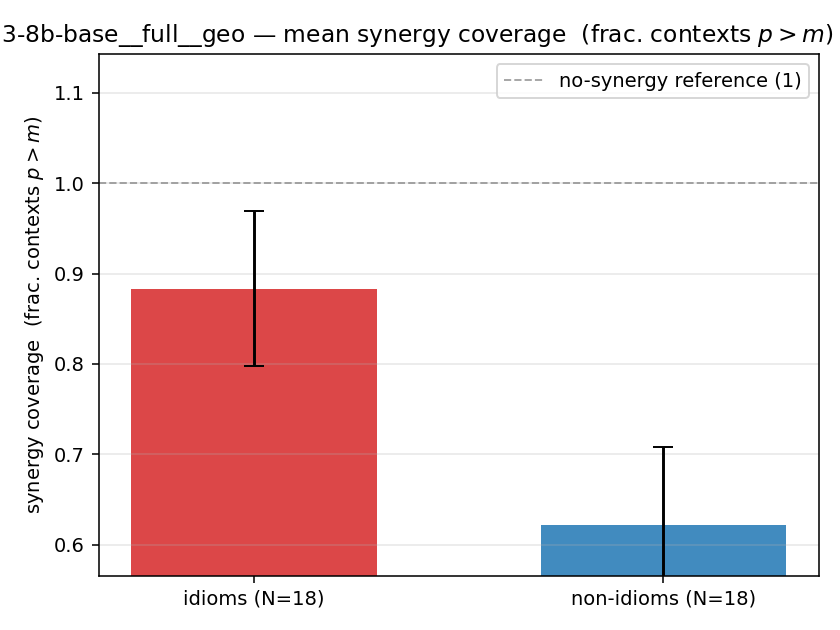 |
| per-idiom (sorted) | 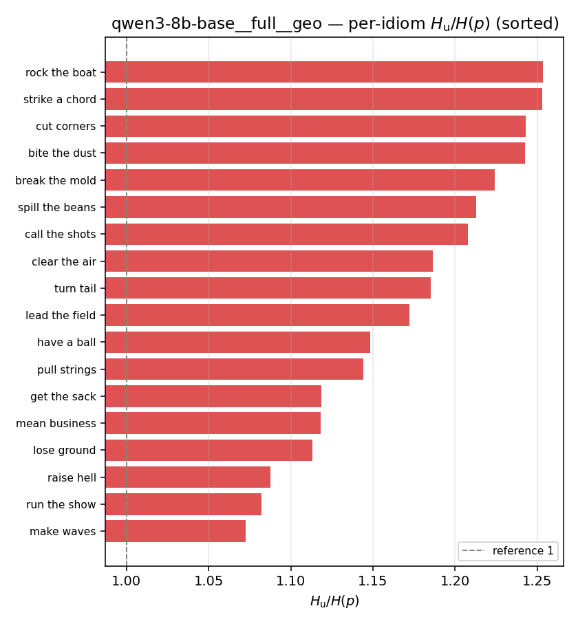 | 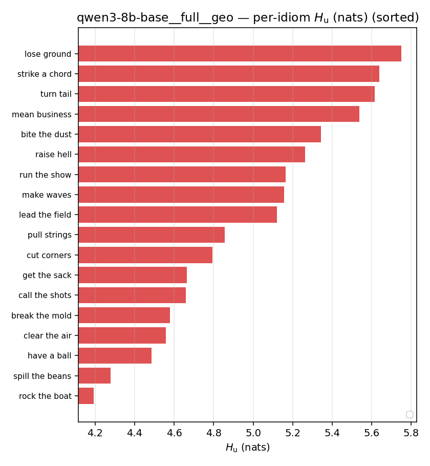 | — (no finite values) | — (no finite values) | 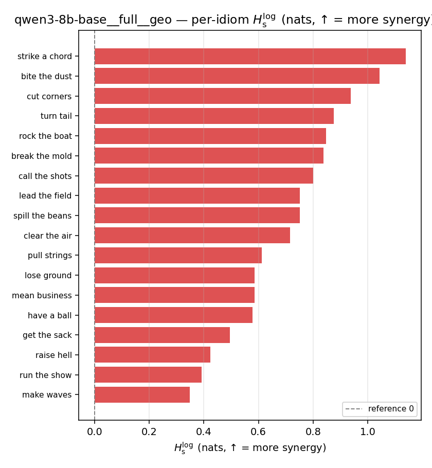 | 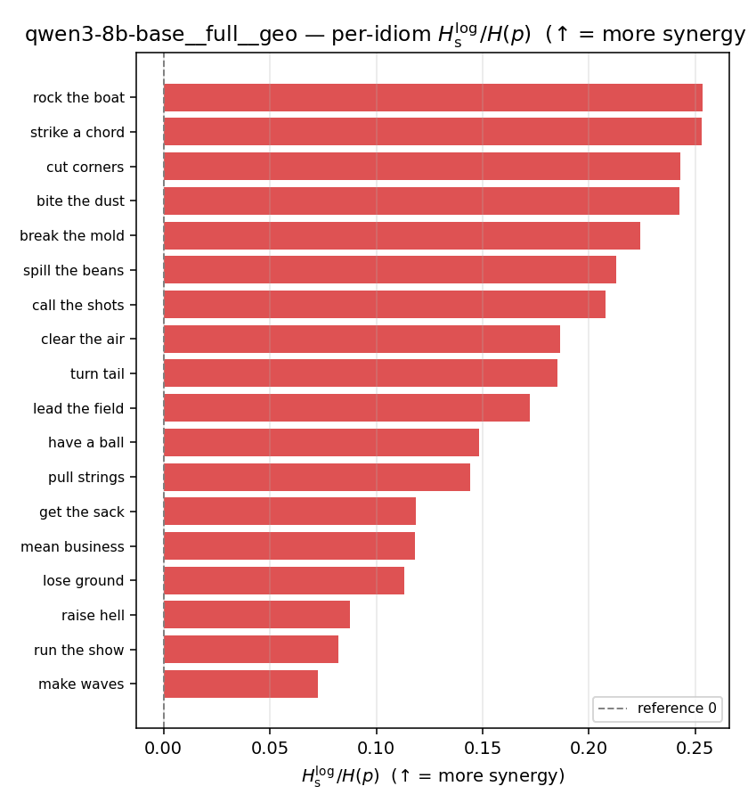 | 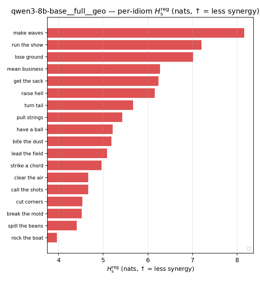 | 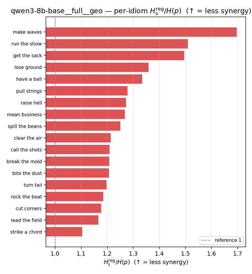 | 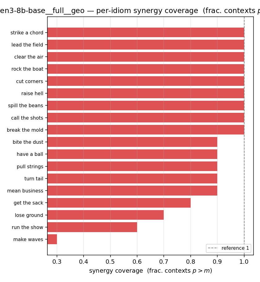 |
qwen3-8b-base · full · joint qwen3-8b-base__full__joint
| Ĥu/Ĥ ↑syn | Ĥu | Ĥs ↓syn | Ĥs/Ĥ ↓syn | Ĥslog ↑syn | Ĥslog/Ĥ ↑syn | Ĥsreg ↓syn | Ĥsreg/Ĥ ↓syn | f̂syn ↑syn | |
|---|---|---|---|---|---|---|---|---|---|
| strip (per-phrase) | 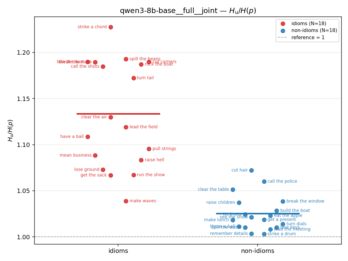 | 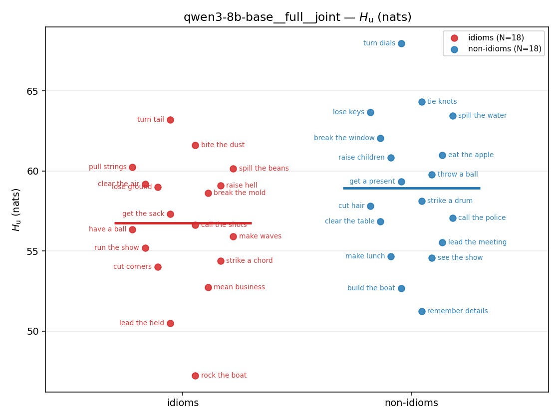 | — (no finite values) | — (no finite values) | 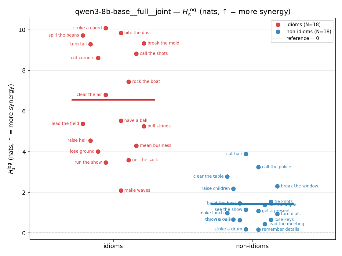 | 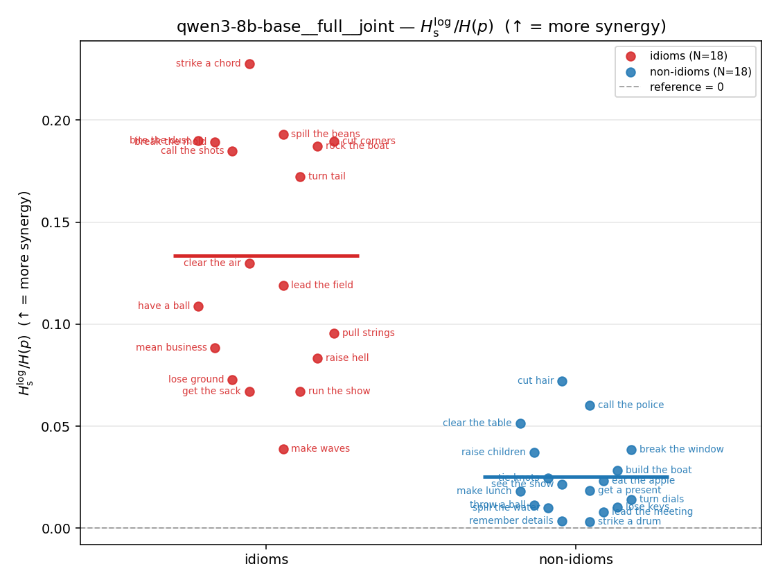 | 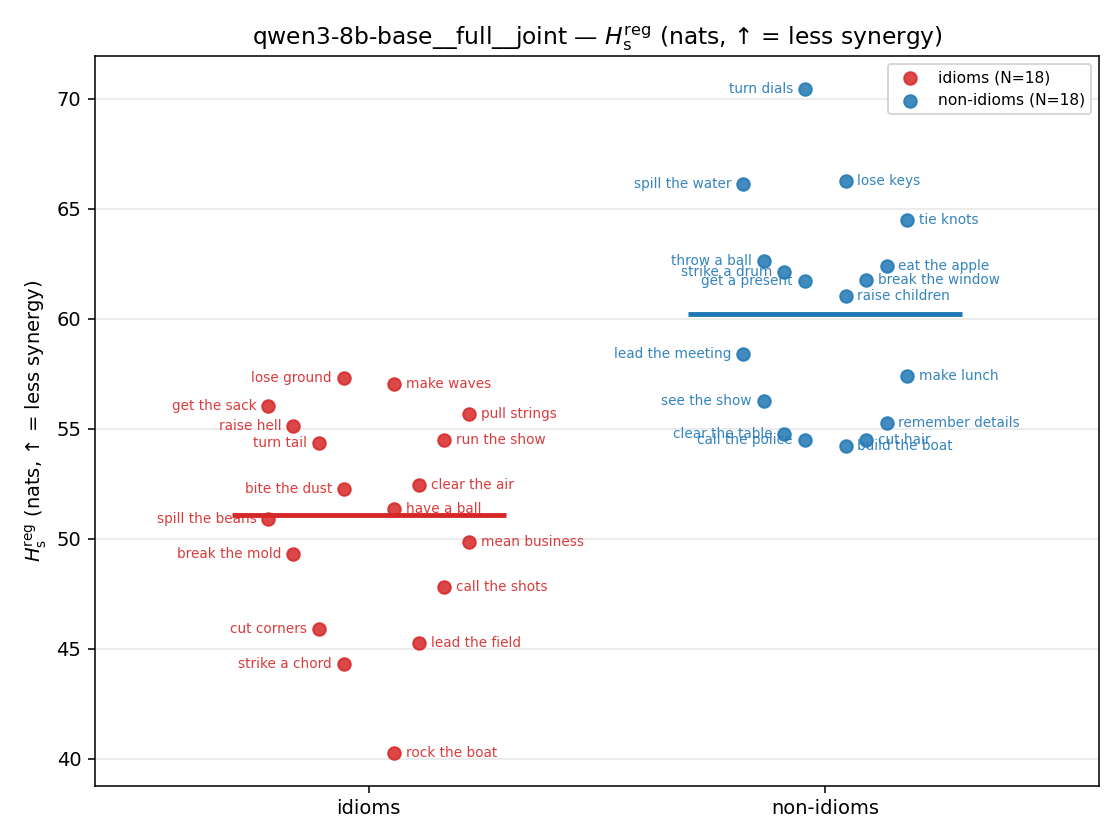 | 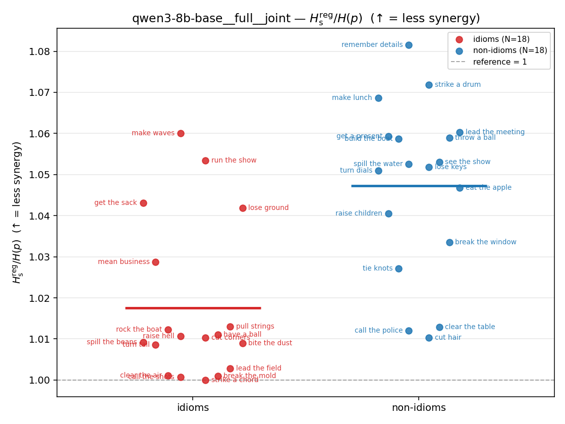 | 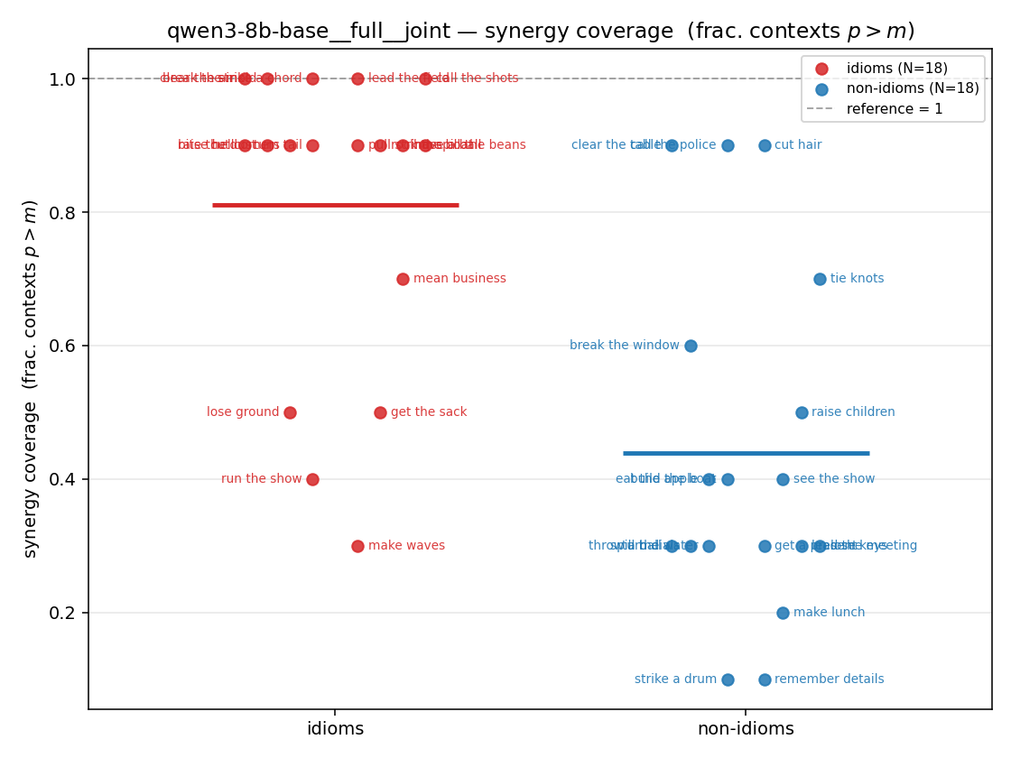 |
| mean ± 95% CI | 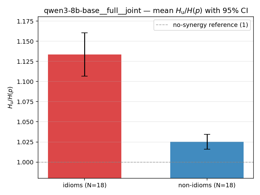 | 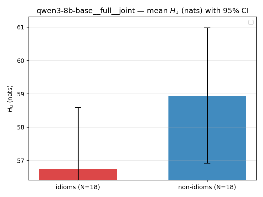 | — (no finite values) | — (no finite values) | 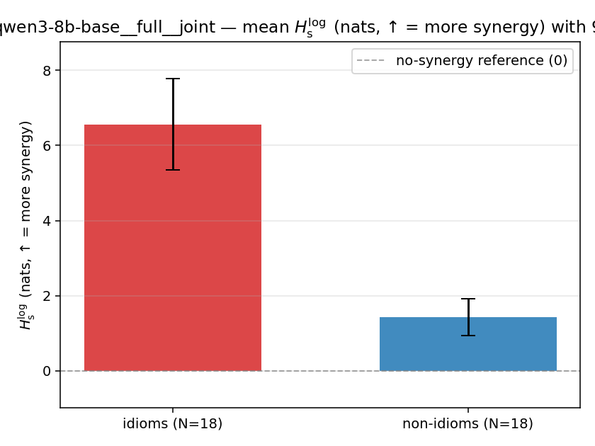 | 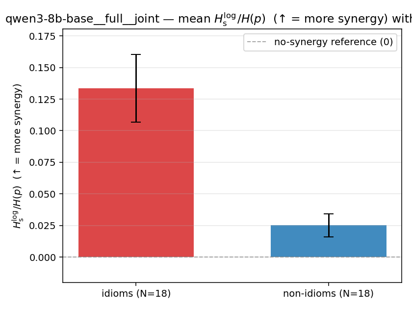 | 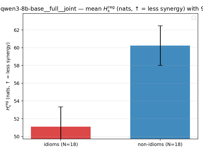 | 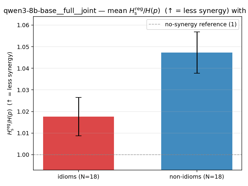 | 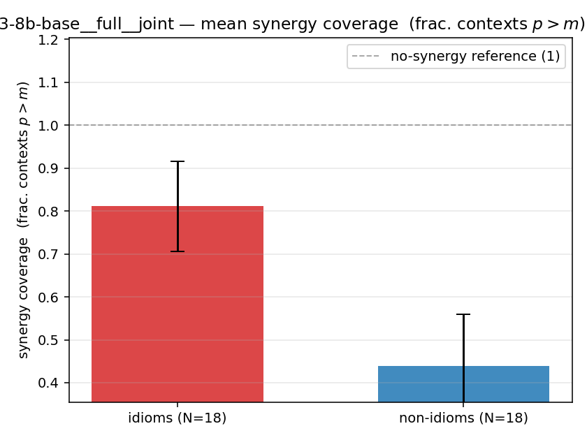 |
| per-idiom (sorted) | 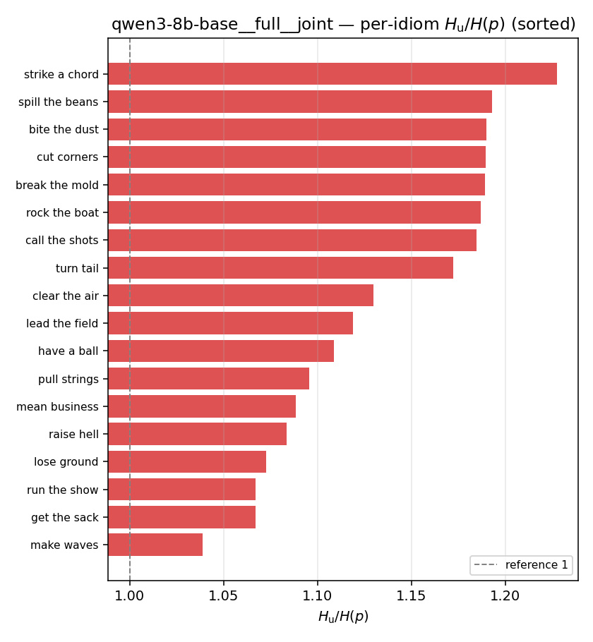 | 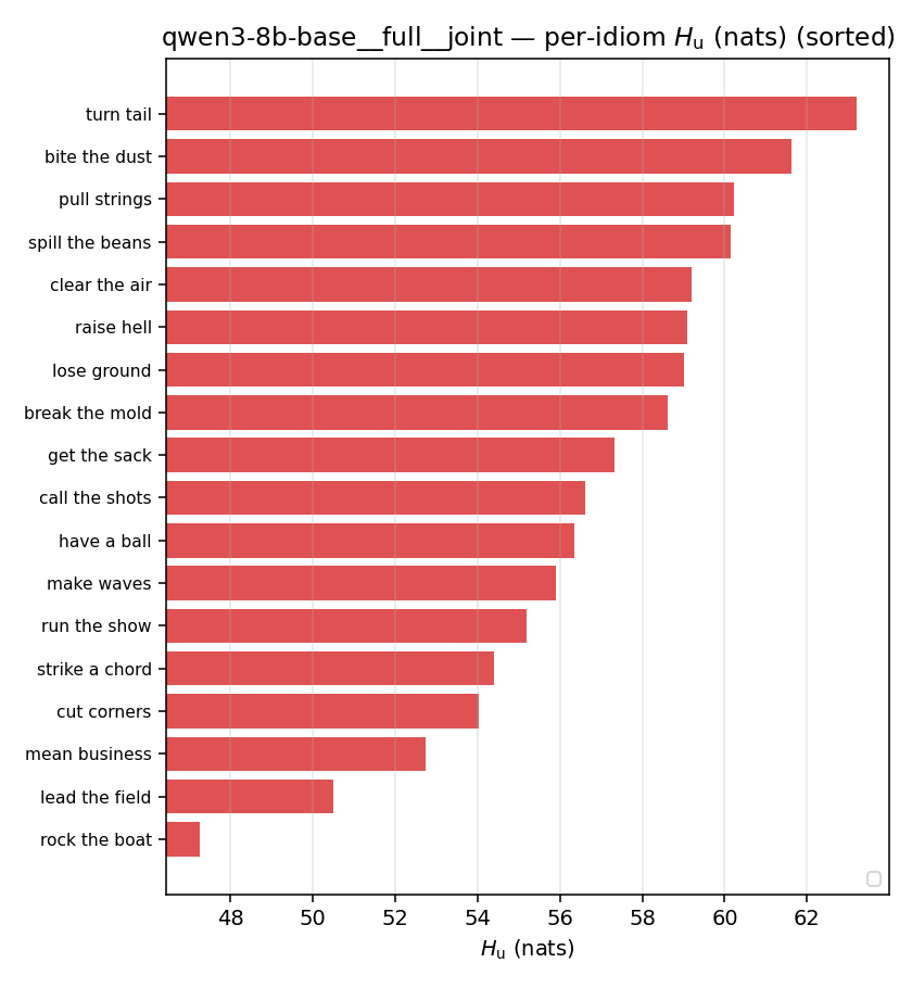 | — (no finite values) | — (no finite values) | 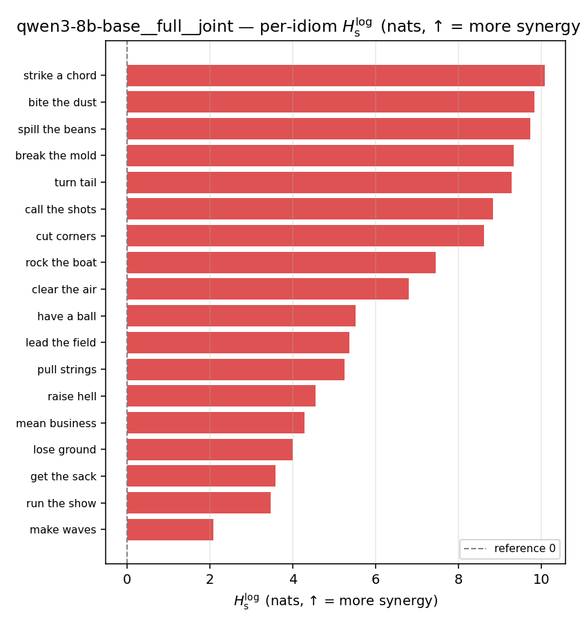 | 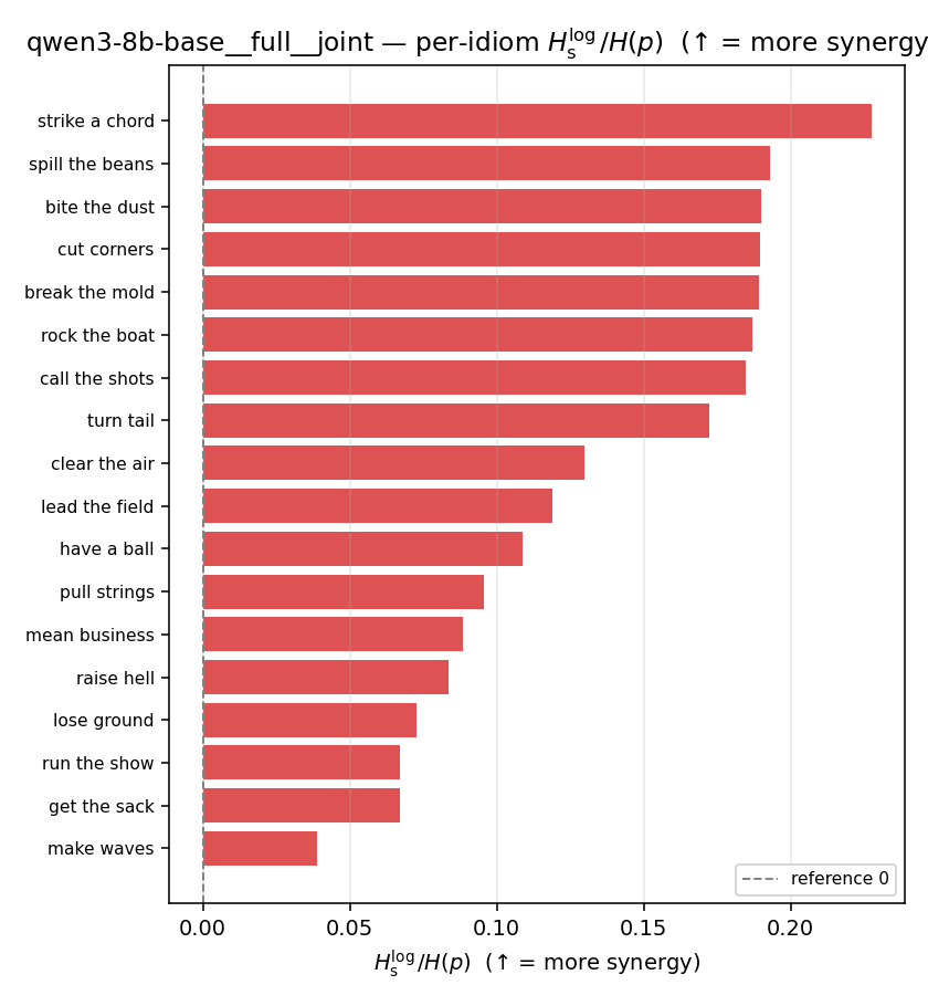 | 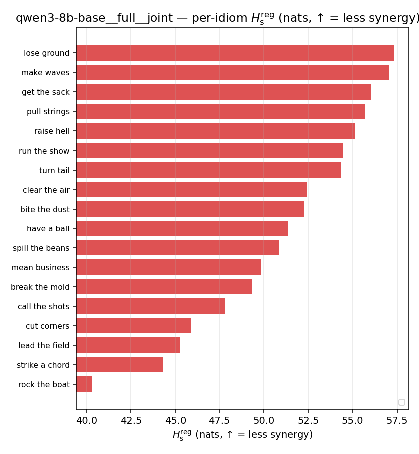 | 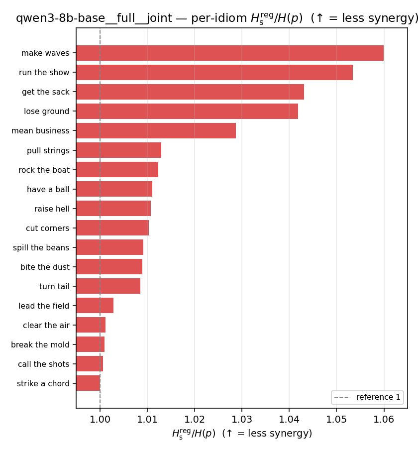 | 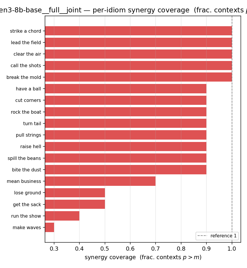 |
qwen3-8b — per-config figures
3×9 grid of figure-type × metric (↑syn / ↓syn in a header = the metric increases / decreases with synergy; definitions on the entropies page). Tables scroll horizontally; “— (no finite values)” marks Ĥs/ratio_s panels where every phrase was +inf. Click to zoom.
qwen3-8b · medial · geo qwen3-8b__medial__geo
| Ĥu/Ĥ ↑syn | Ĥu | Ĥs ↓syn | Ĥs/Ĥ ↓syn | Ĥslog ↑syn | Ĥslog/Ĥ ↑syn | Ĥsreg ↓syn | Ĥsreg/Ĥ ↓syn | f̂syn ↑syn | |
|---|---|---|---|---|---|---|---|---|---|
| strip (per-phrase) | 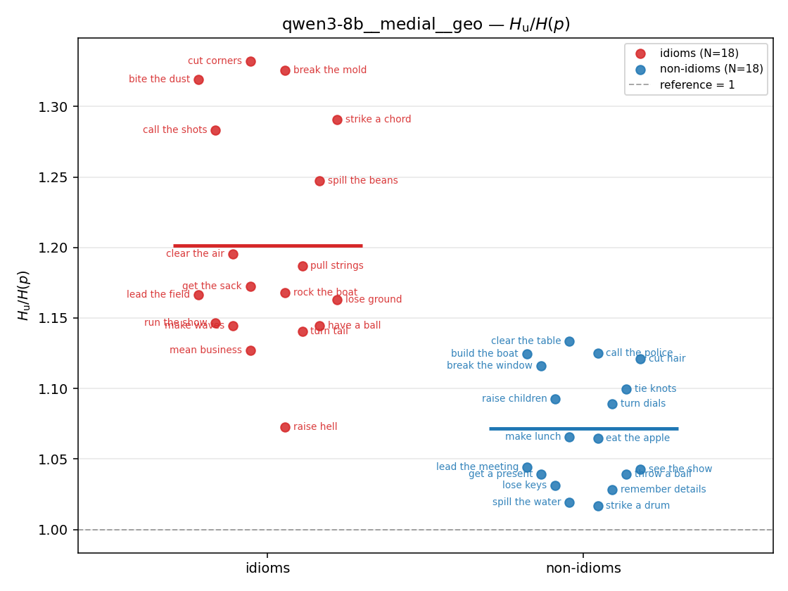 | 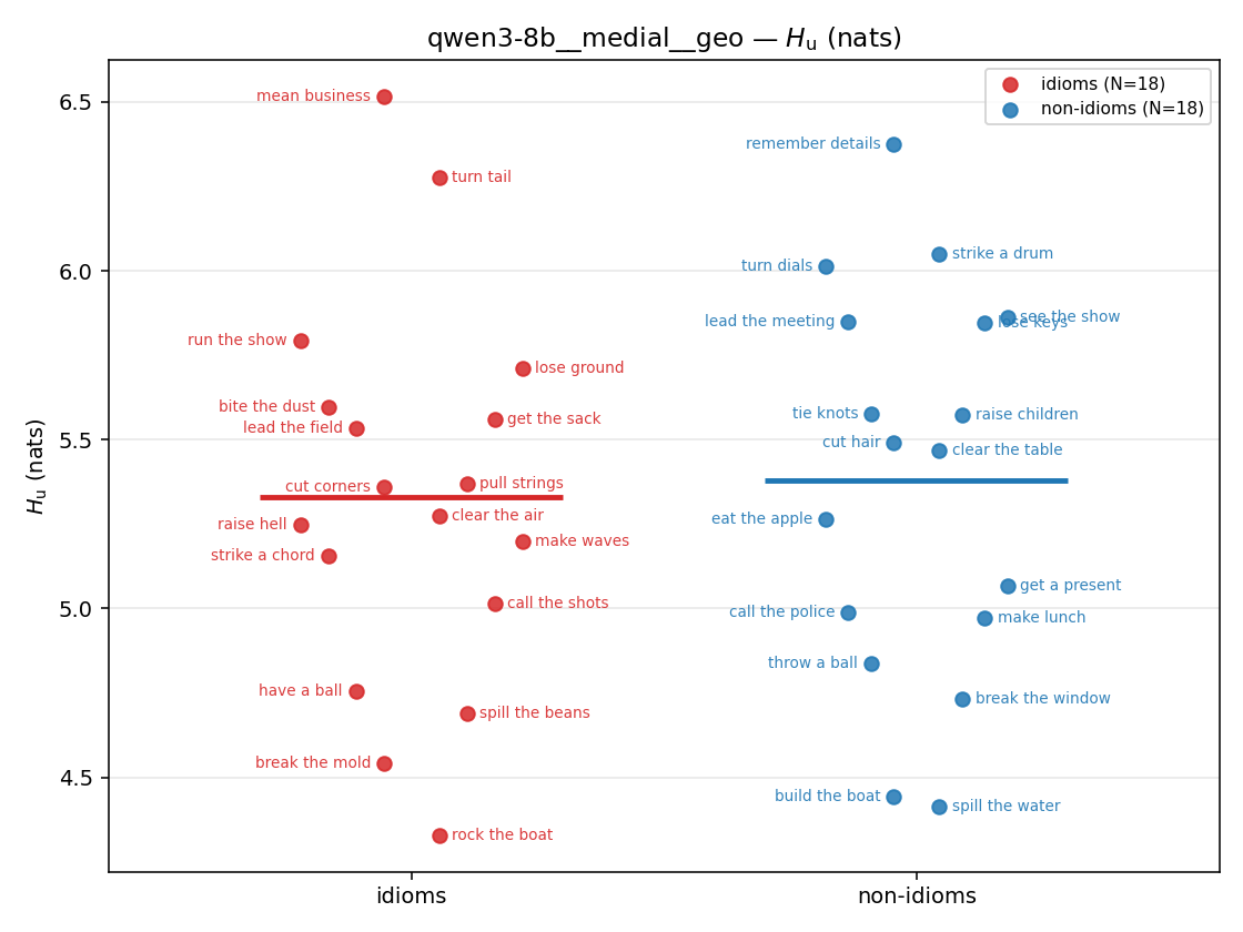 | 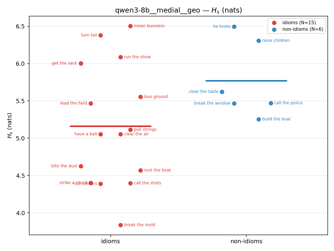 | 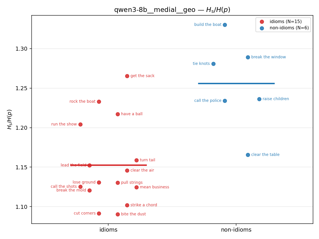 | 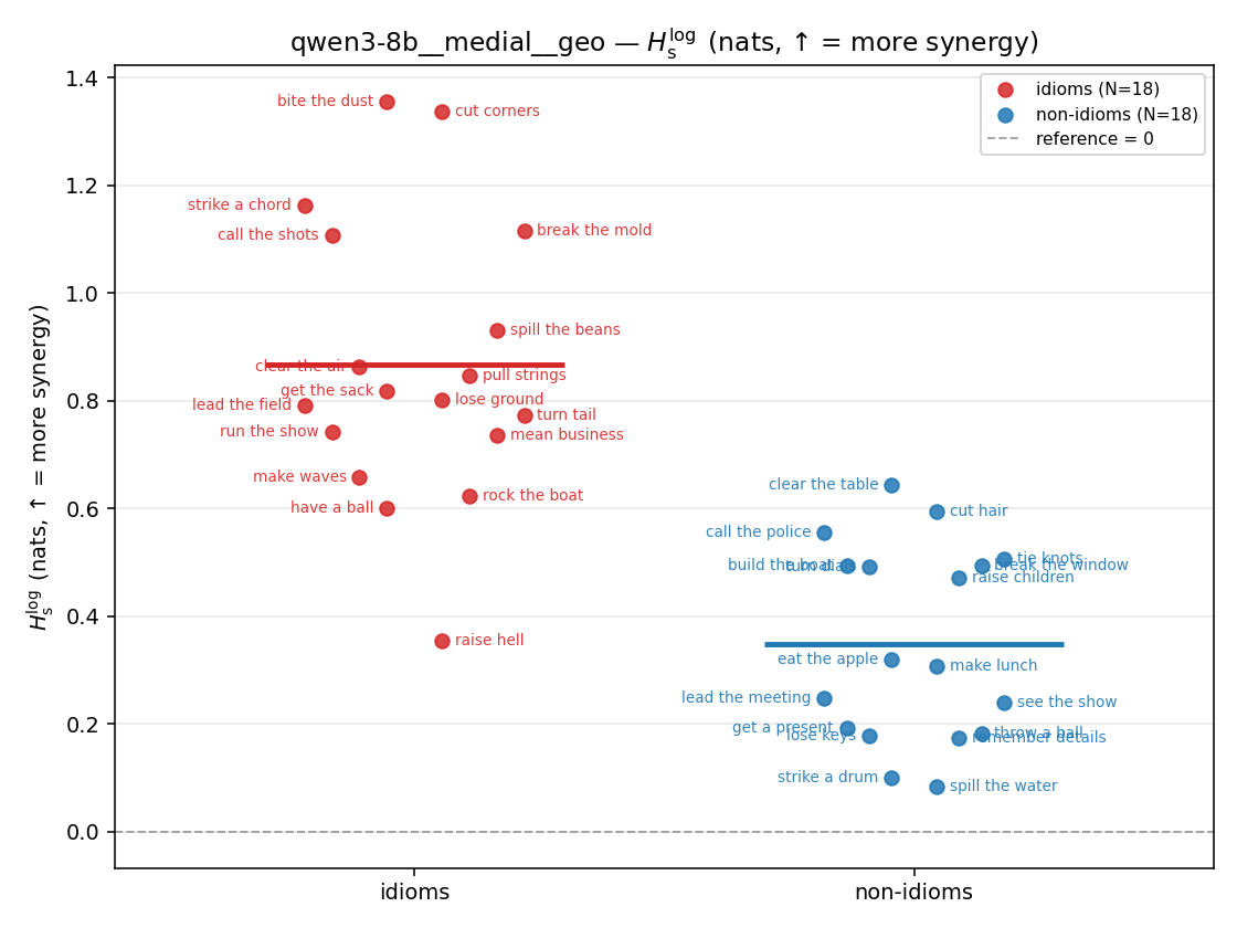 | 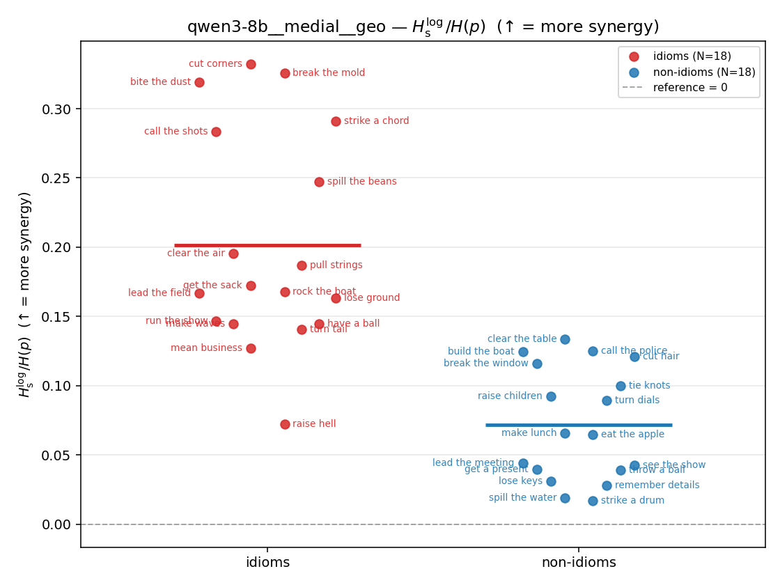 | 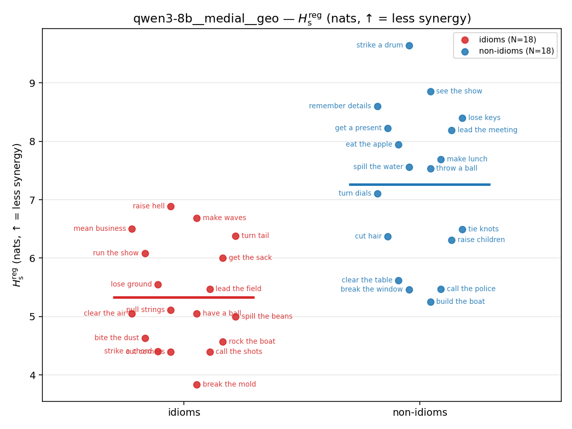 | 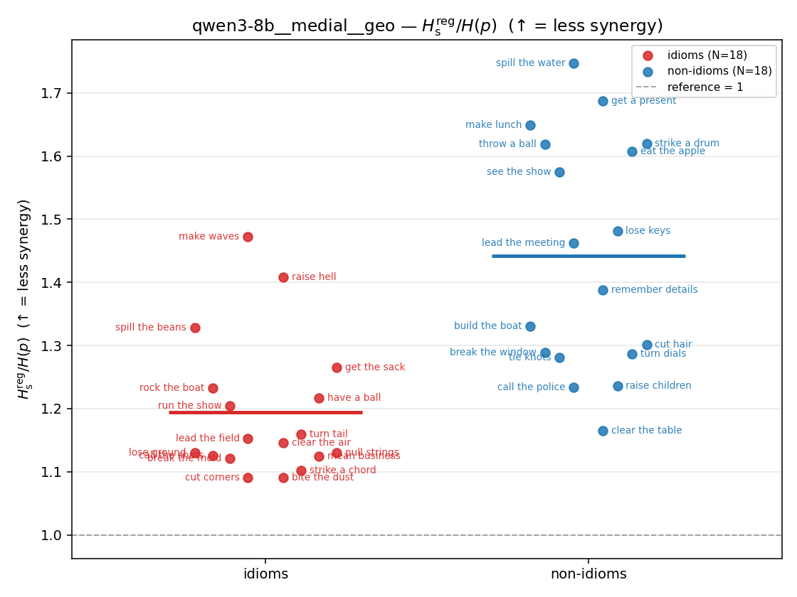 | 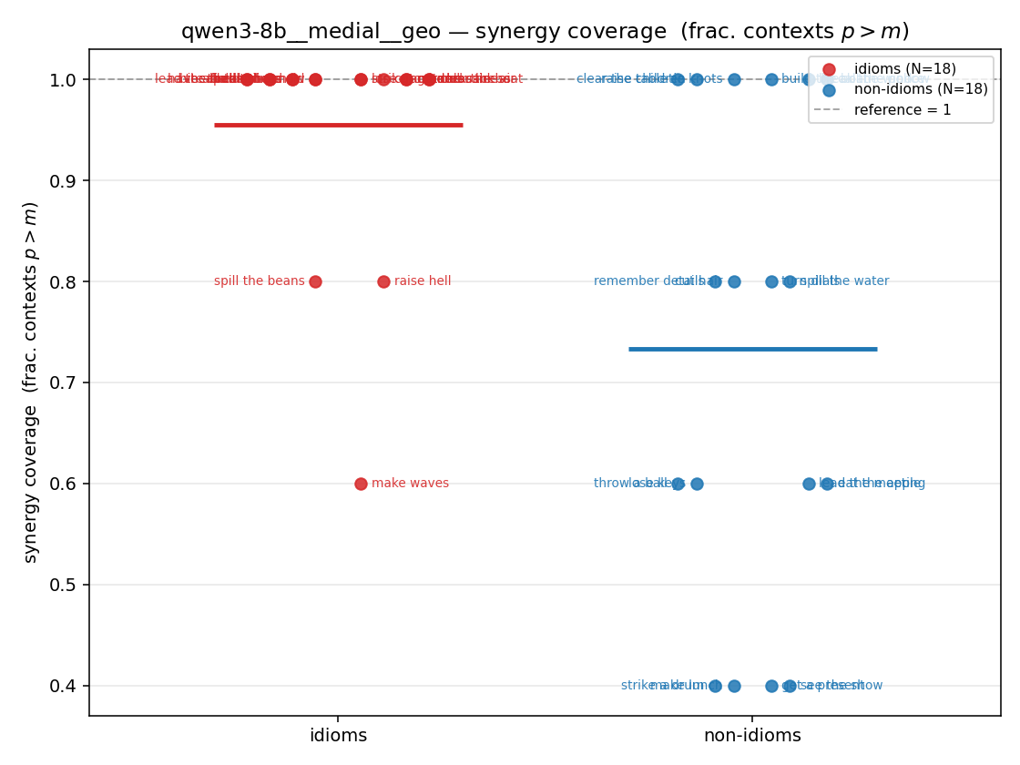 |
| mean ± 95% CI | 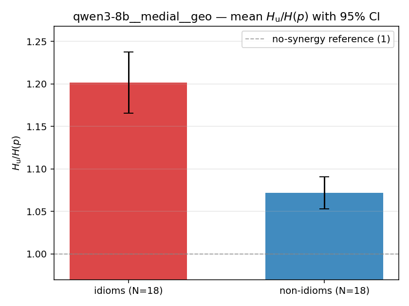 | 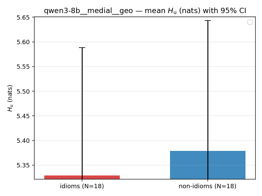 | 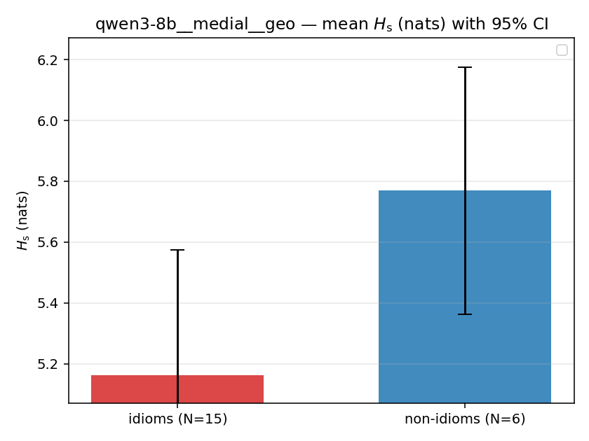 | 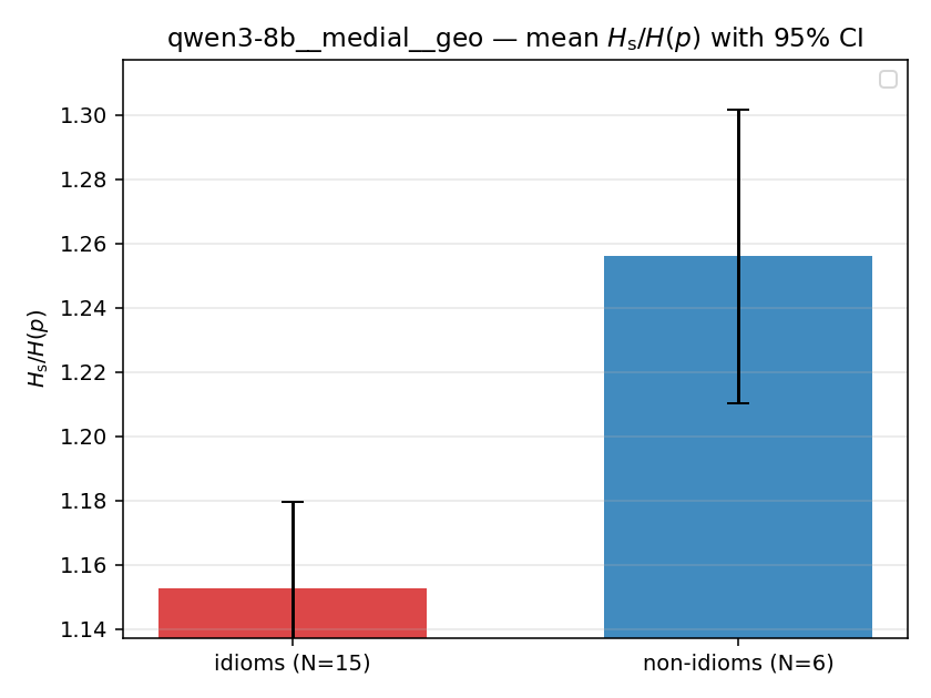 | 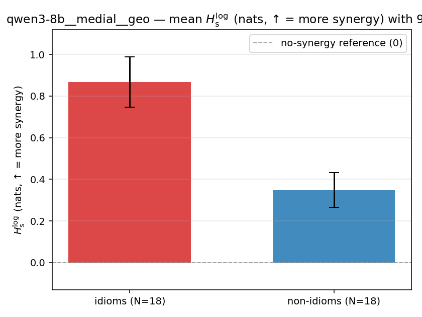 | 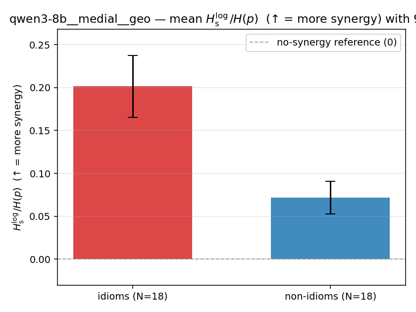 | 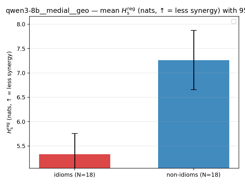 | 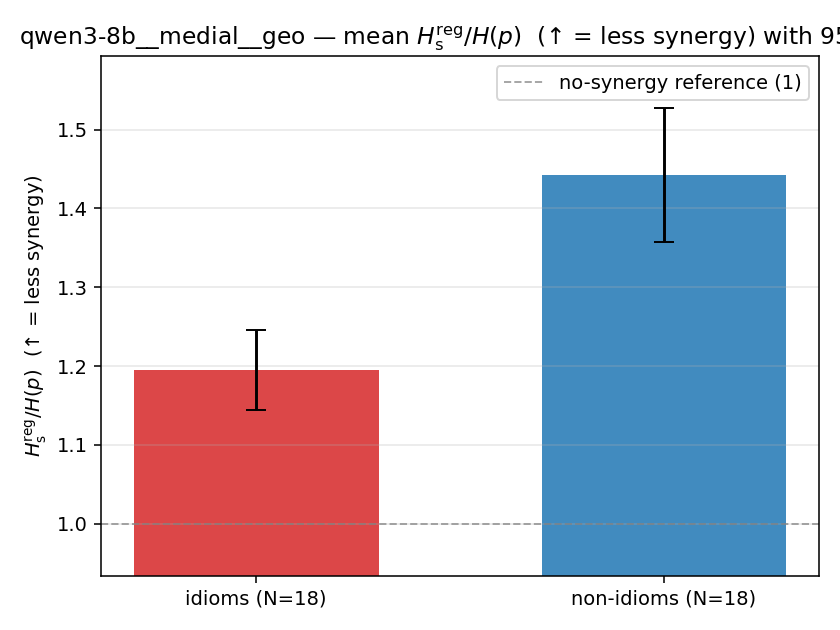 | 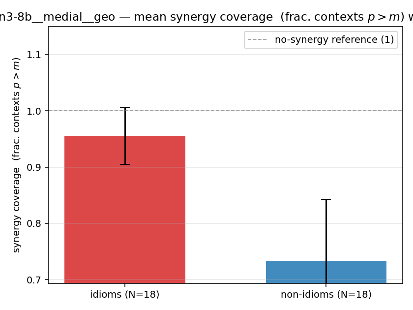 |
| per-idiom (sorted) | 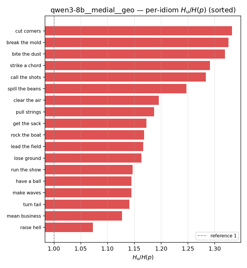 | 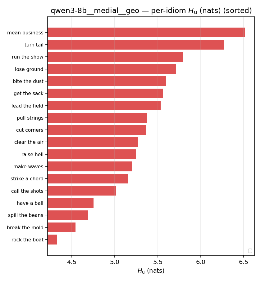 | 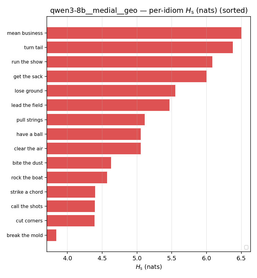 | 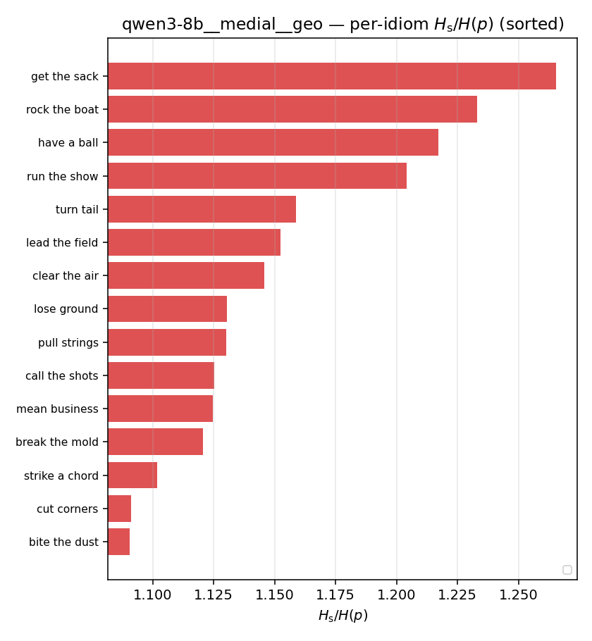 | 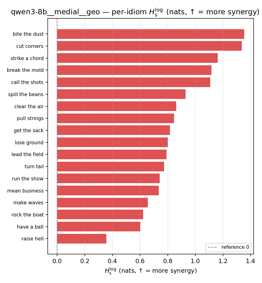 | 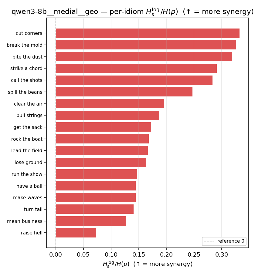 | 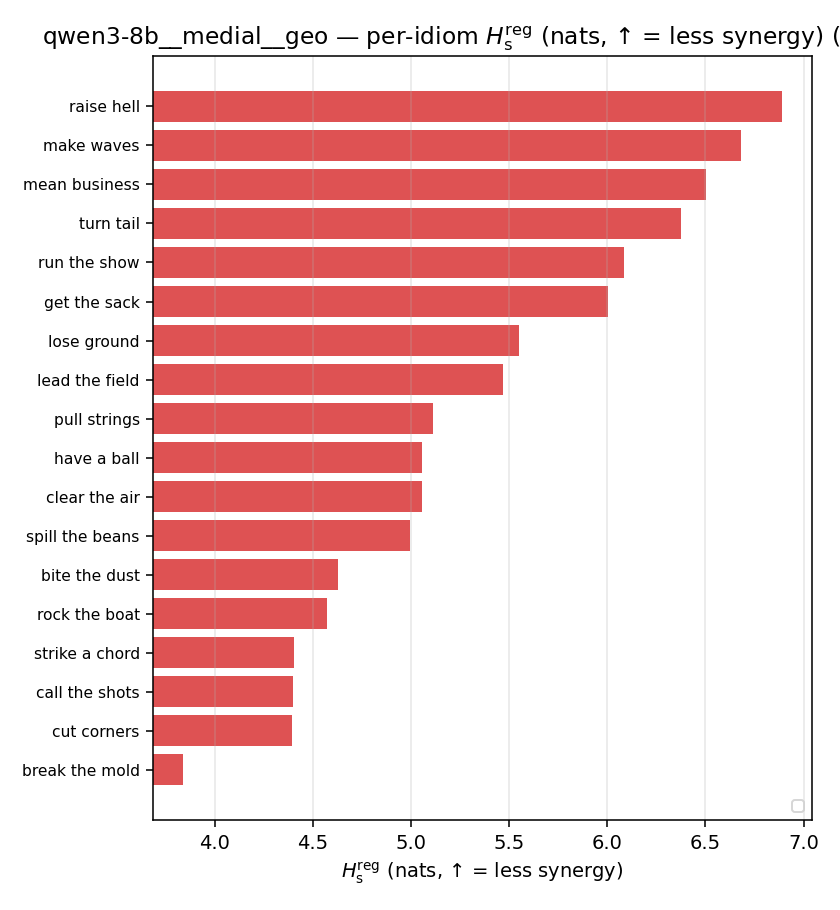 | 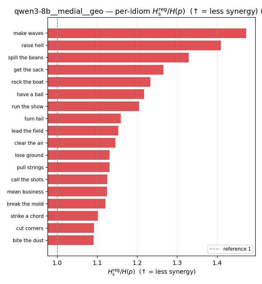 | 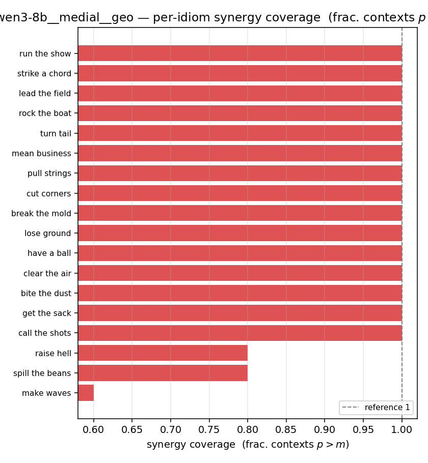 |
qwen3-8b · medial · joint qwen3-8b__medial__joint
| Ĥu/Ĥ ↑syn | Ĥu | Ĥs ↓syn | Ĥs/Ĥ ↓syn | Ĥslog ↑syn | Ĥslog/Ĥ ↑syn | Ĥsreg ↓syn | Ĥsreg/Ĥ ↓syn | f̂syn ↑syn | |
|---|---|---|---|---|---|---|---|---|---|
| strip (per-phrase) | 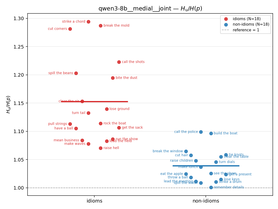 | 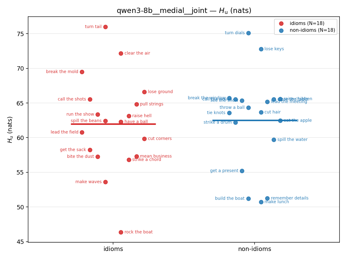 | 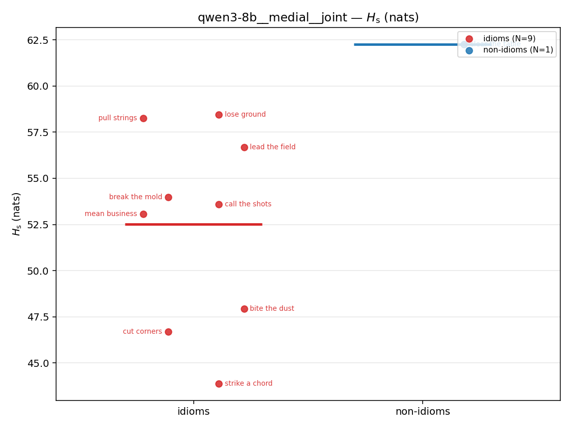 | 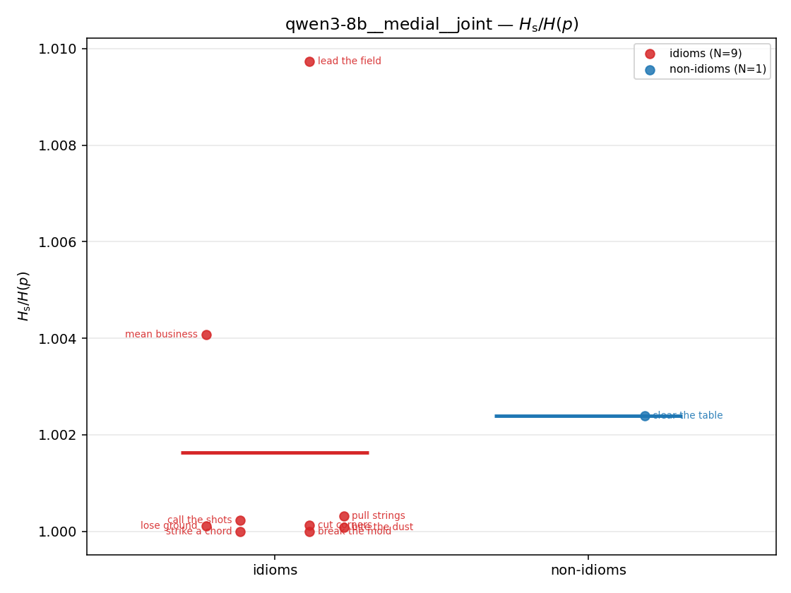 | 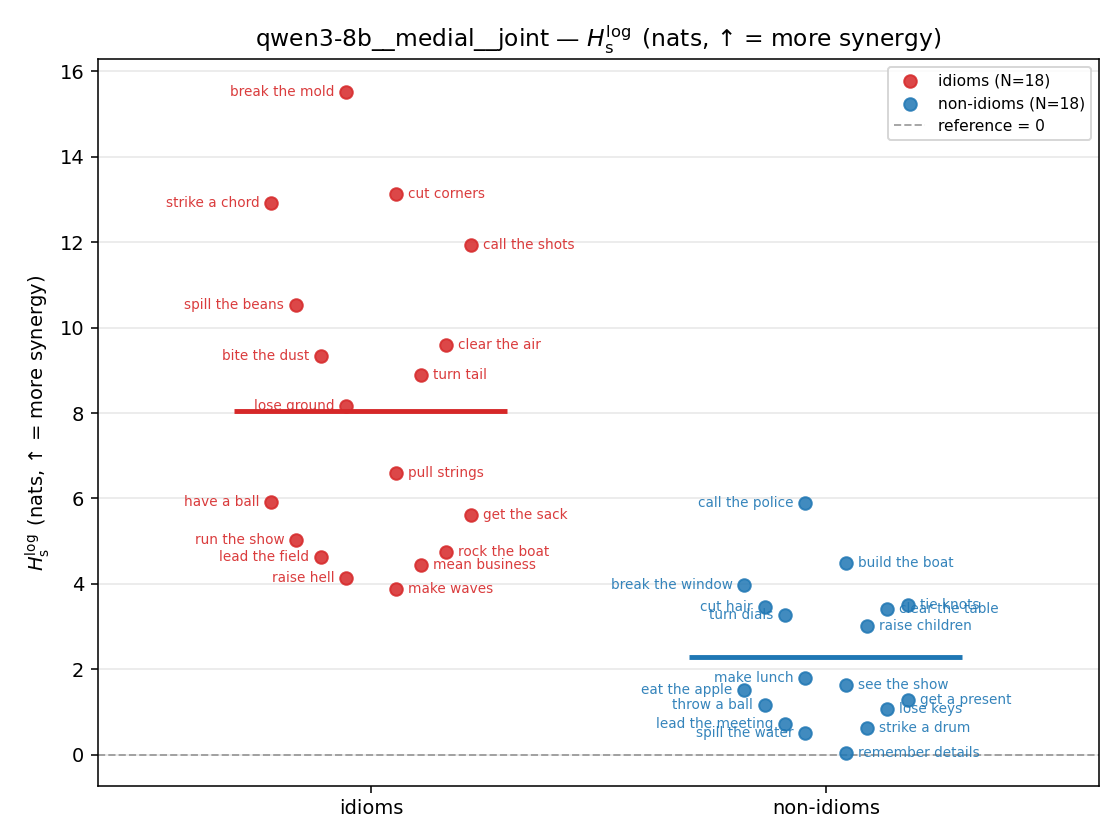 | 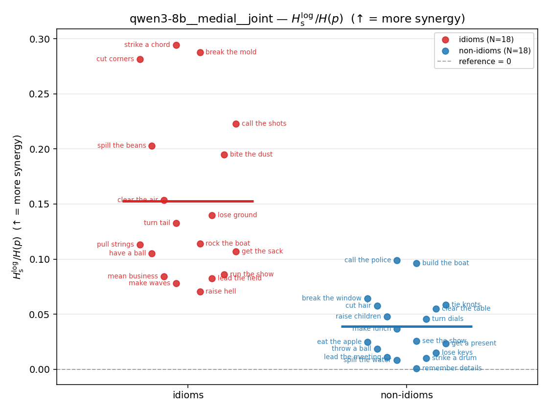 | 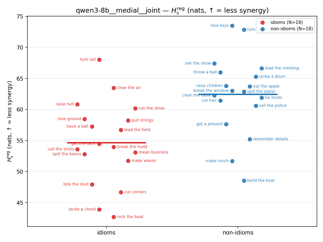 | 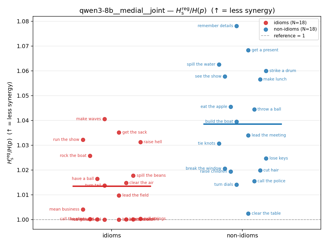 | 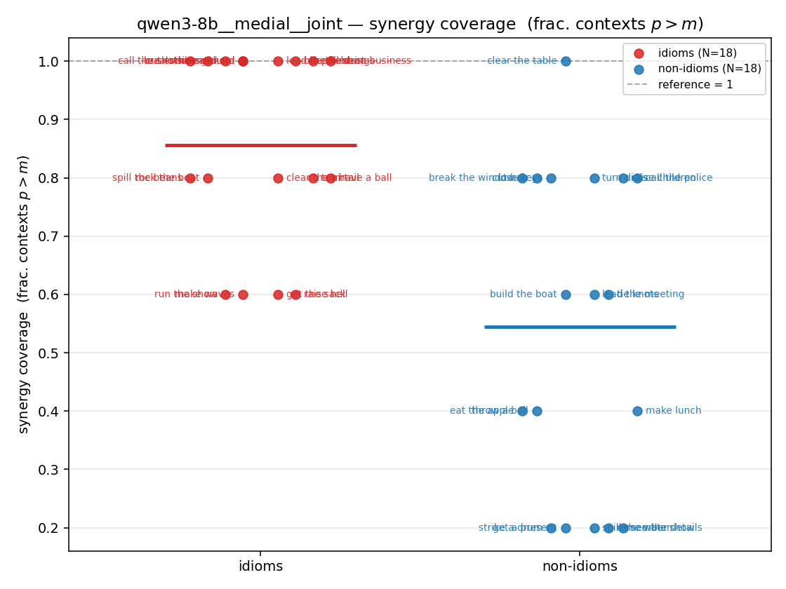 |
| mean ± 95% CI | 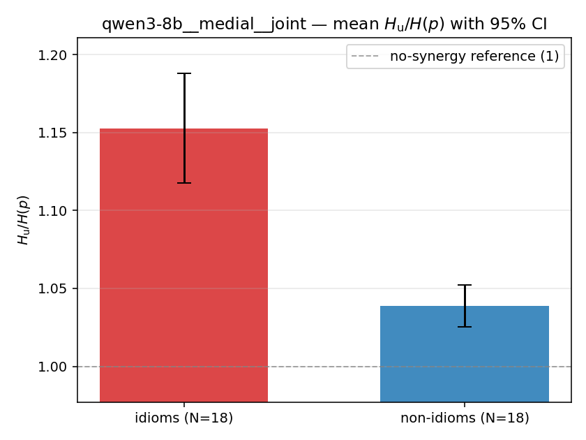 | 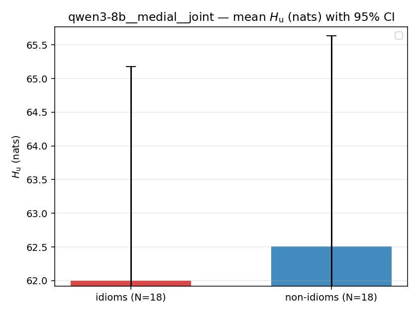 | 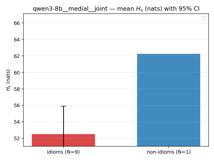 | 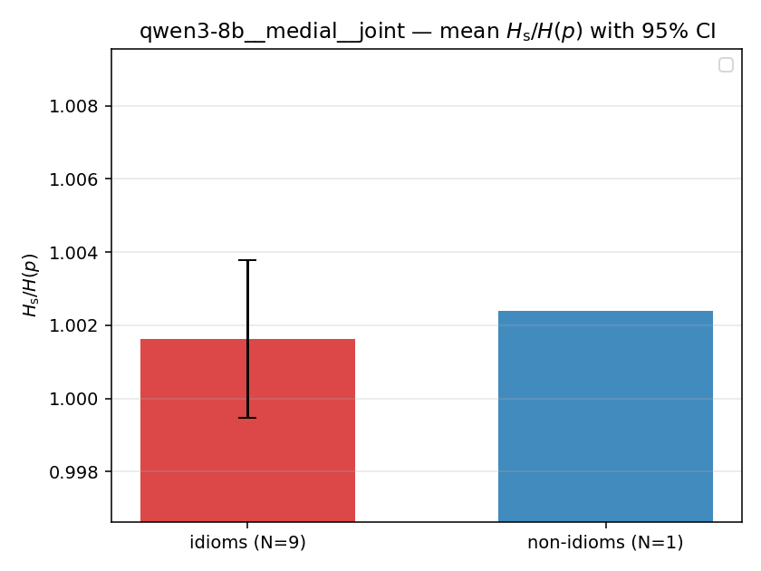 | 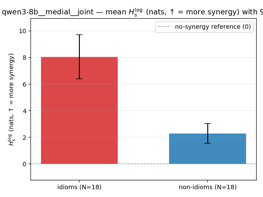 | 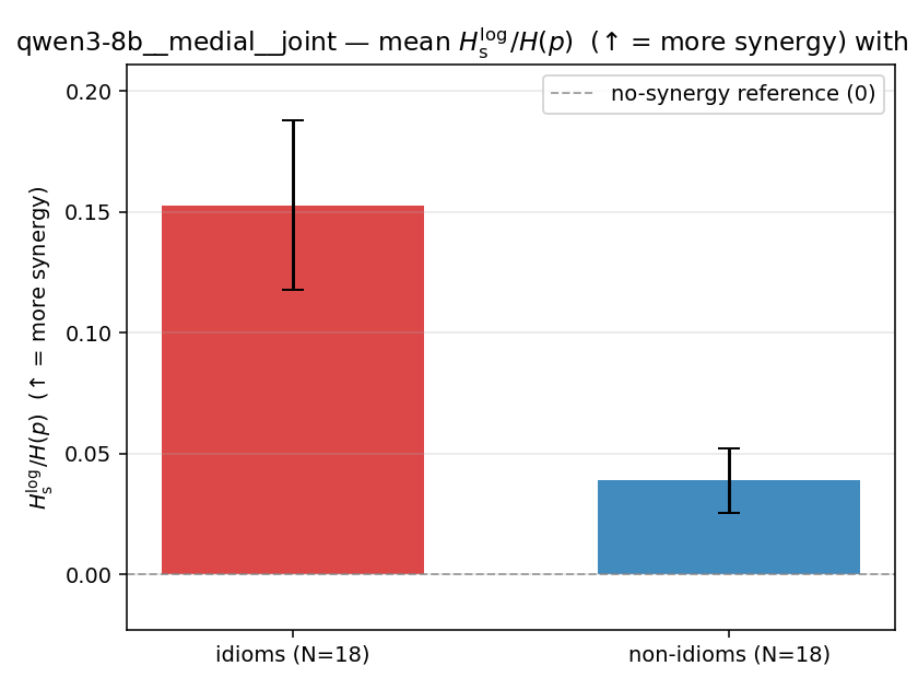 | 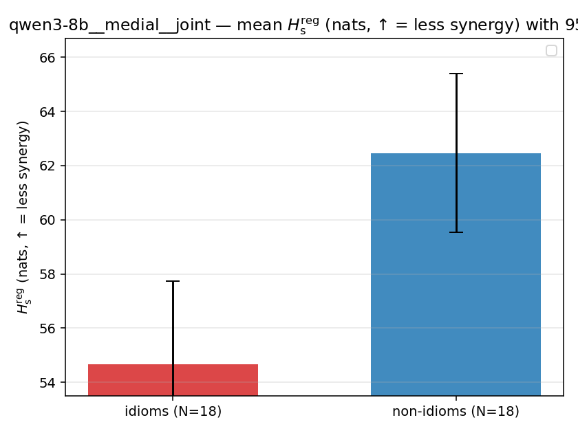 | 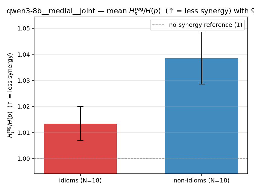 | 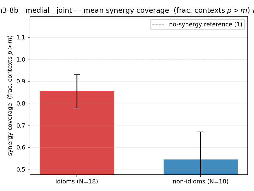 |
| per-idiom (sorted) | 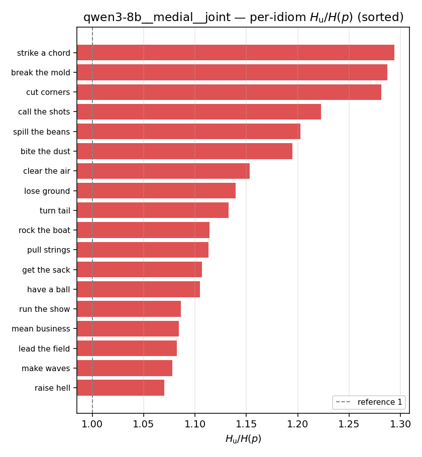 | 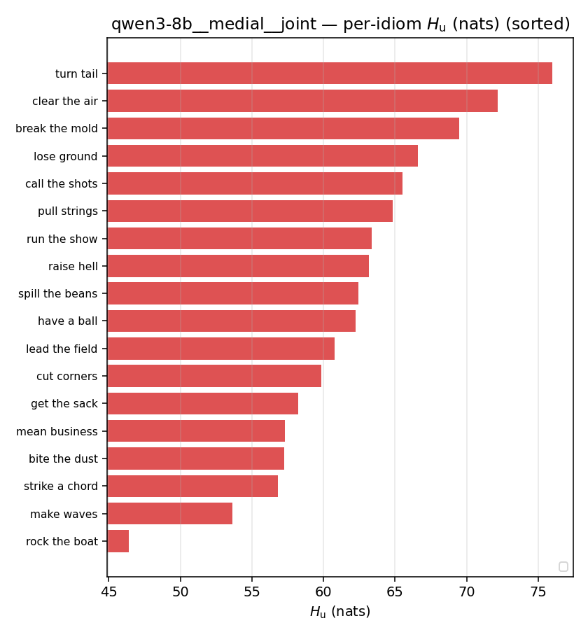 | 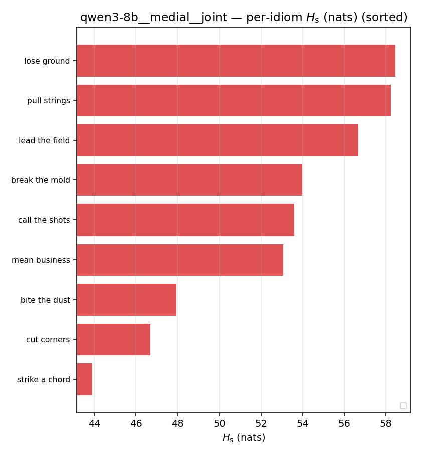 | 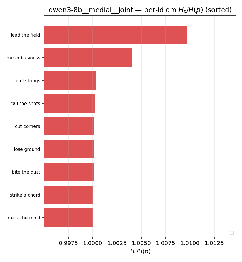 | 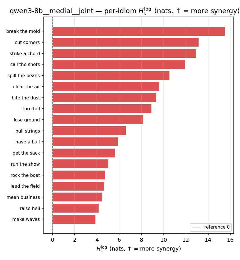 | 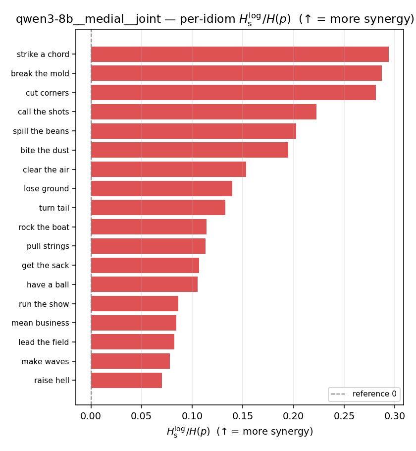 | 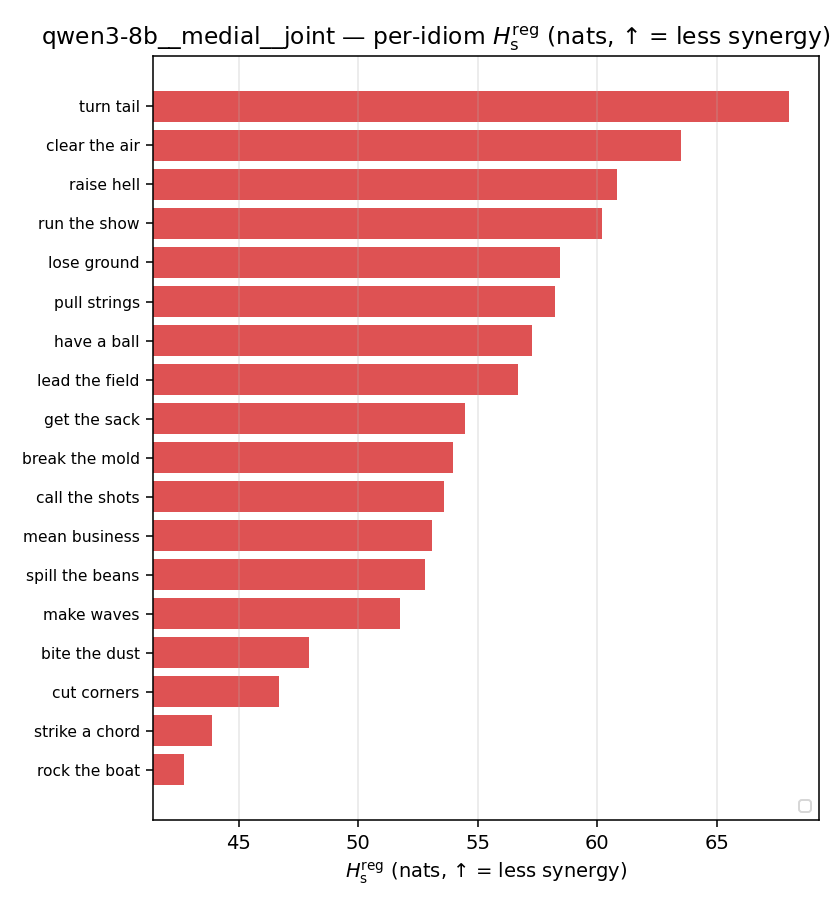 | 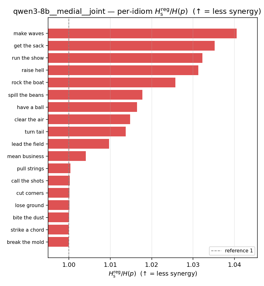 | 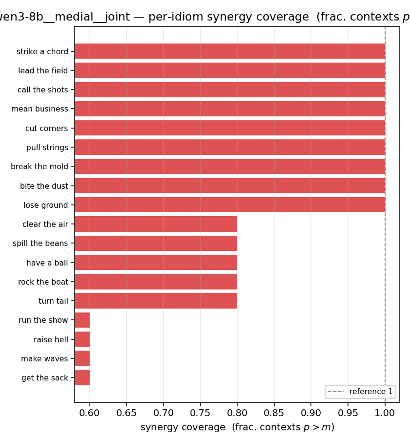 |
qwen3-8b · full · geo qwen3-8b__full__geo
| Ĥu/Ĥ ↑syn | Ĥu | Ĥs ↓syn | Ĥs/Ĥ ↓syn | Ĥslog ↑syn | Ĥslog/Ĥ ↑syn | Ĥsreg ↓syn | Ĥsreg/Ĥ ↓syn | f̂syn ↑syn | |
|---|---|---|---|---|---|---|---|---|---|
| strip (per-phrase) | 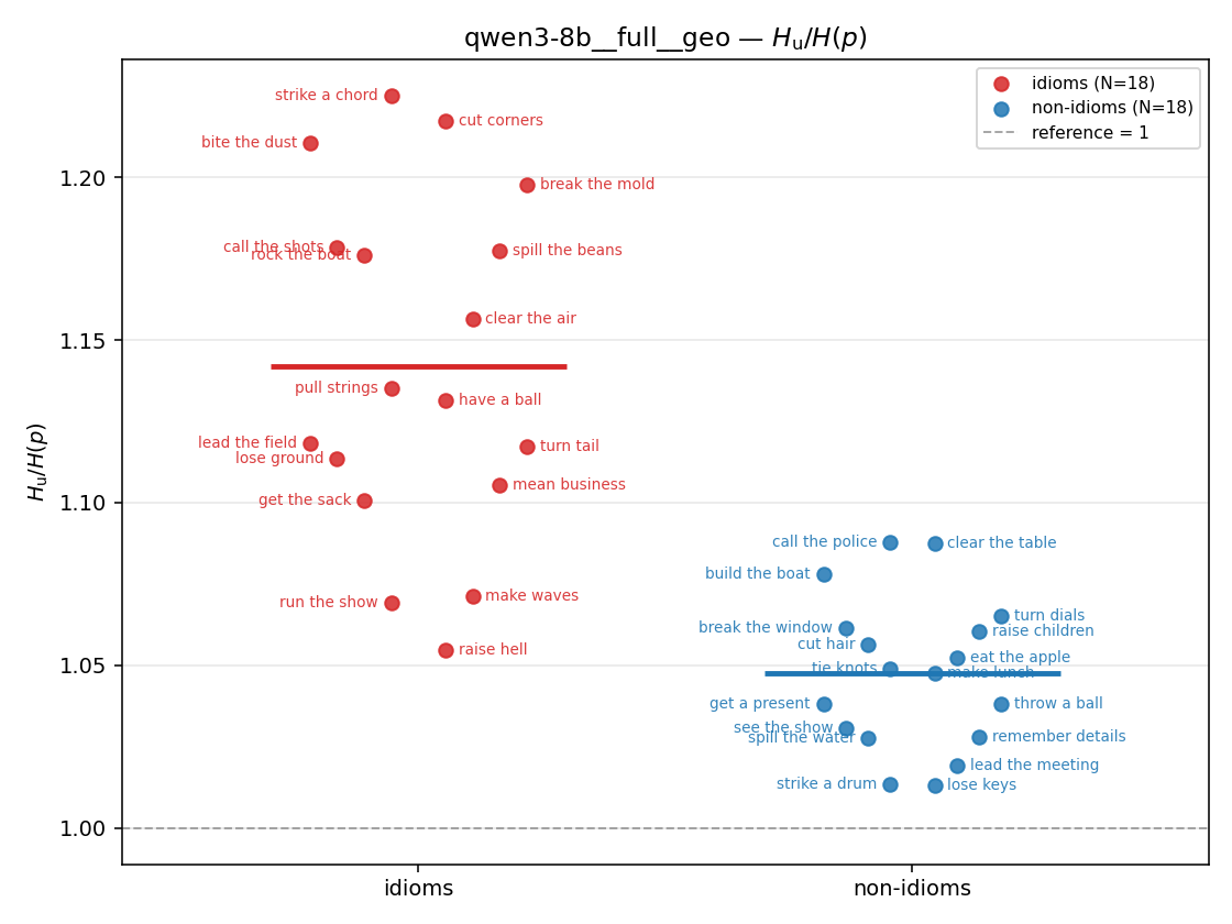 | 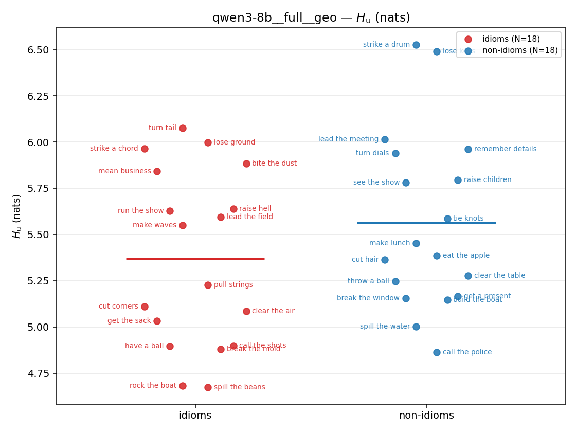 | — (no finite values) | — (no finite values) | 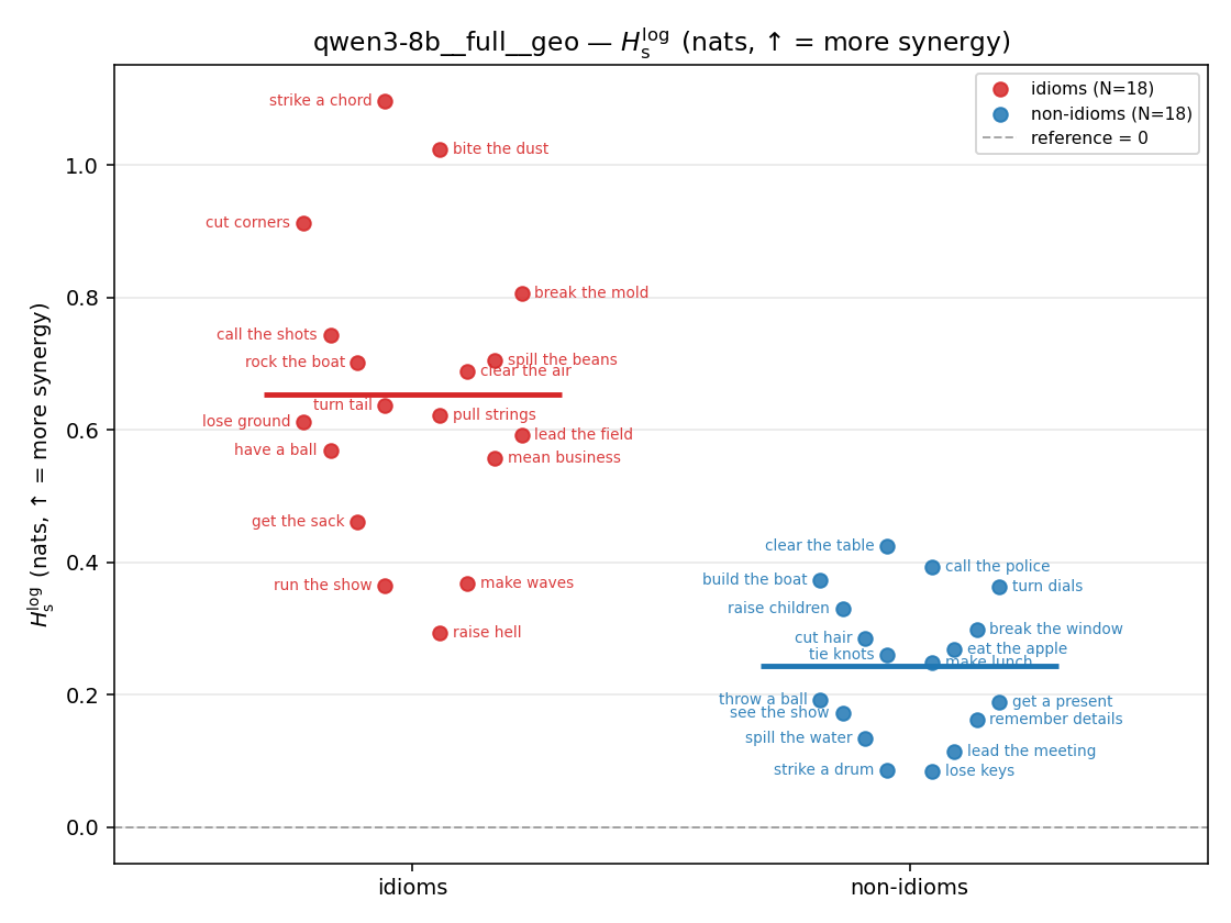 | 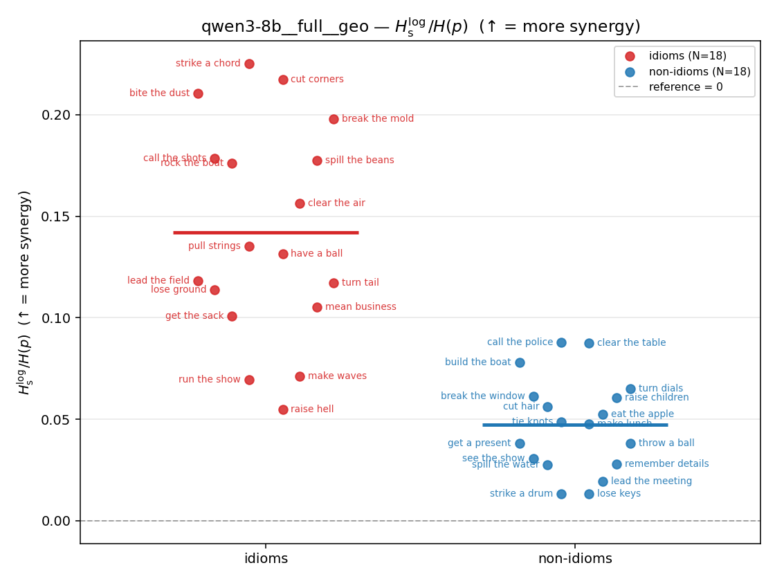 | 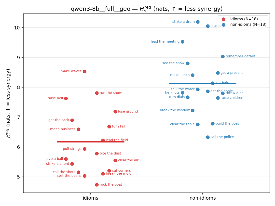 | 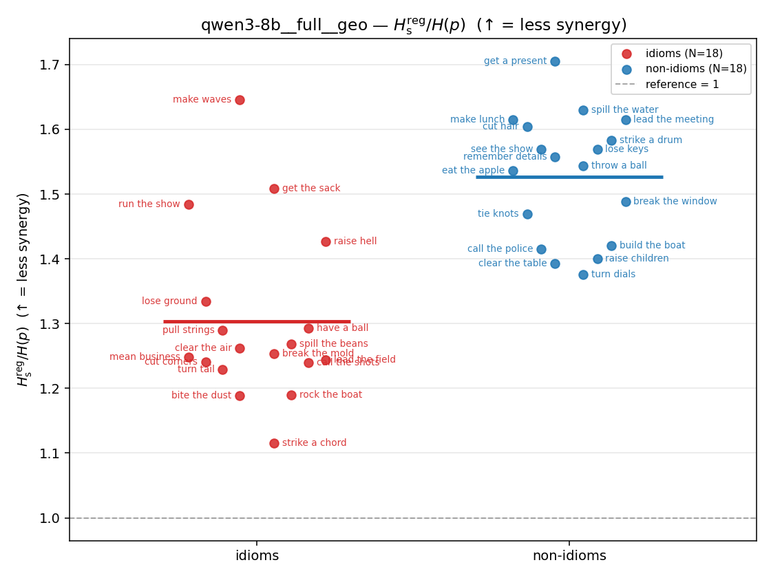 | 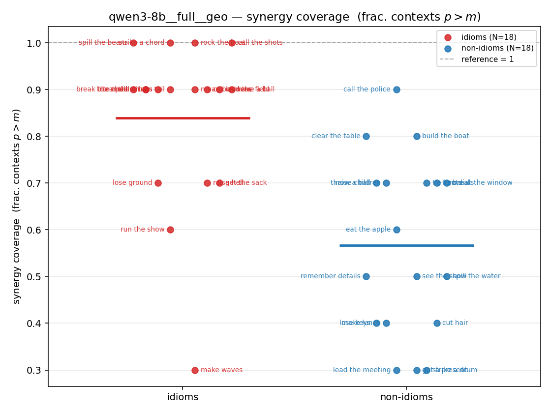 |
| mean ± 95% CI | 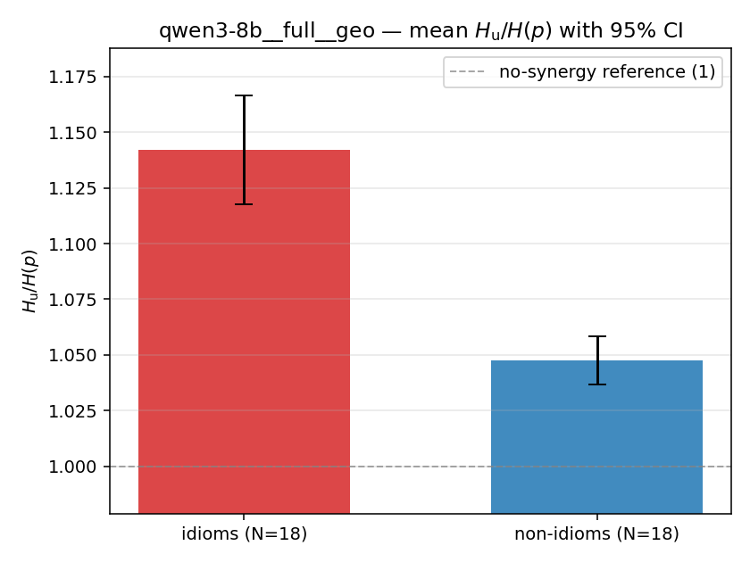 | 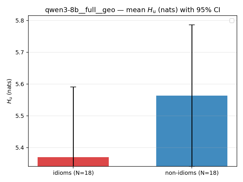 | — (no finite values) | — (no finite values) | 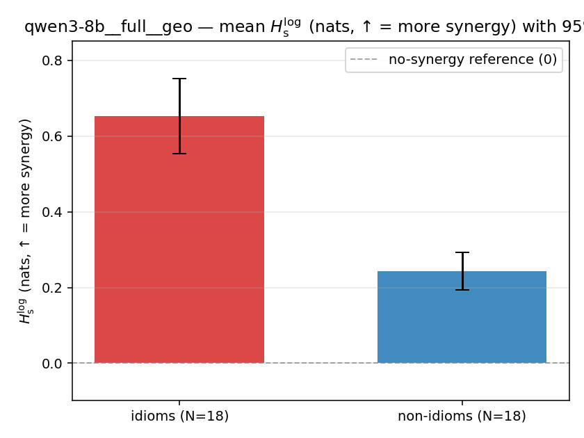 | 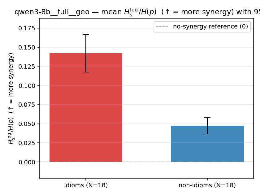 | 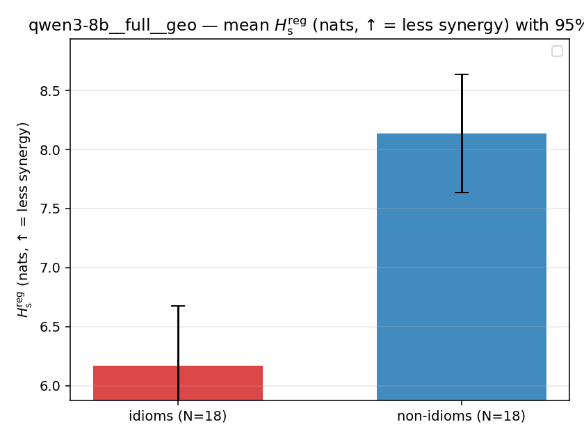 | 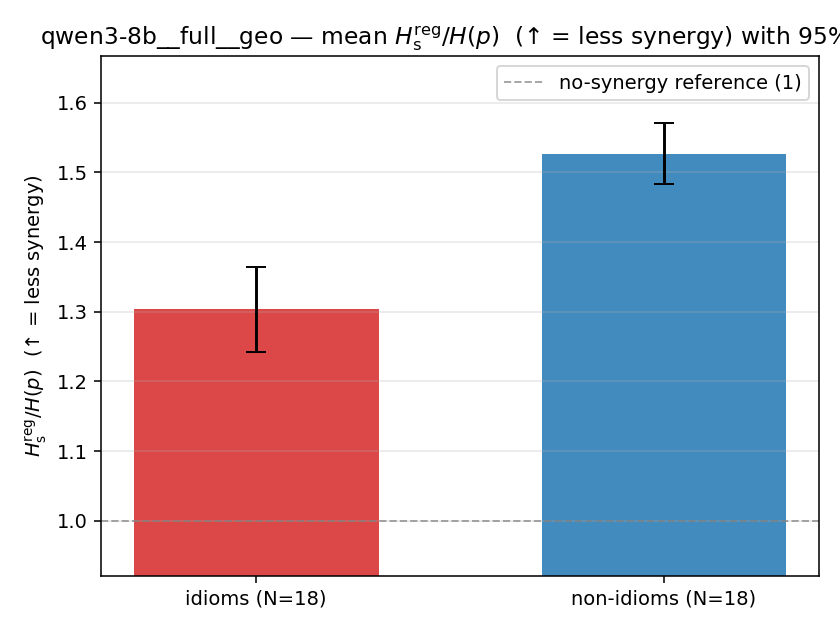 | 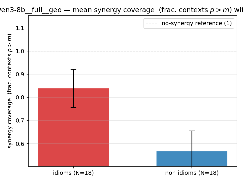 |
| per-idiom (sorted) | 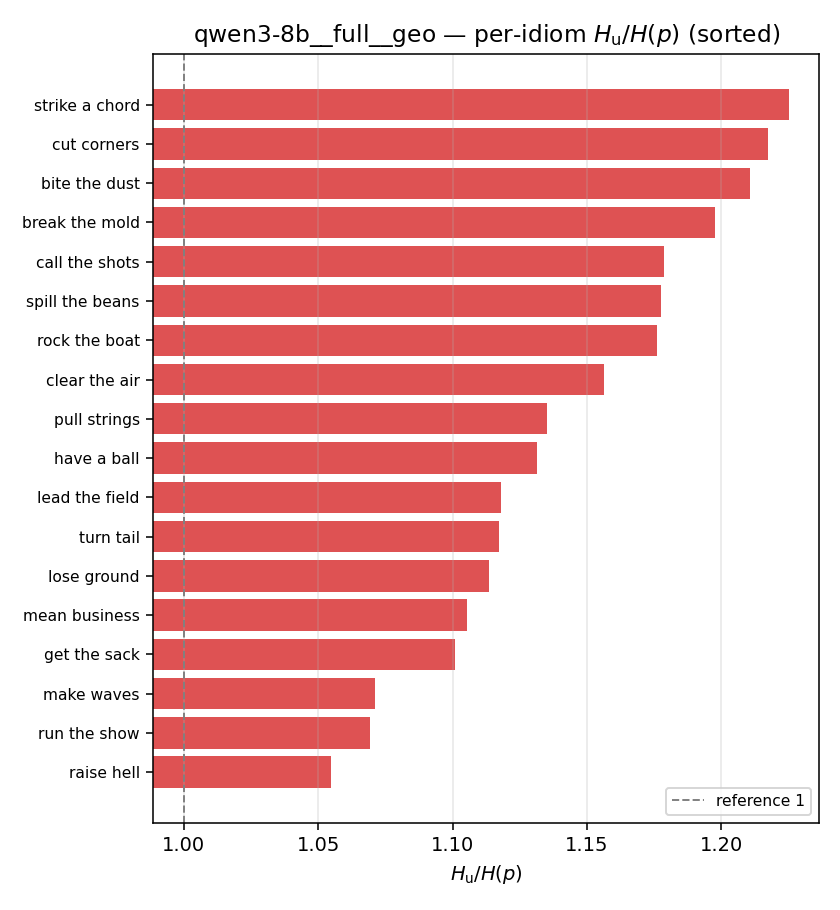 | 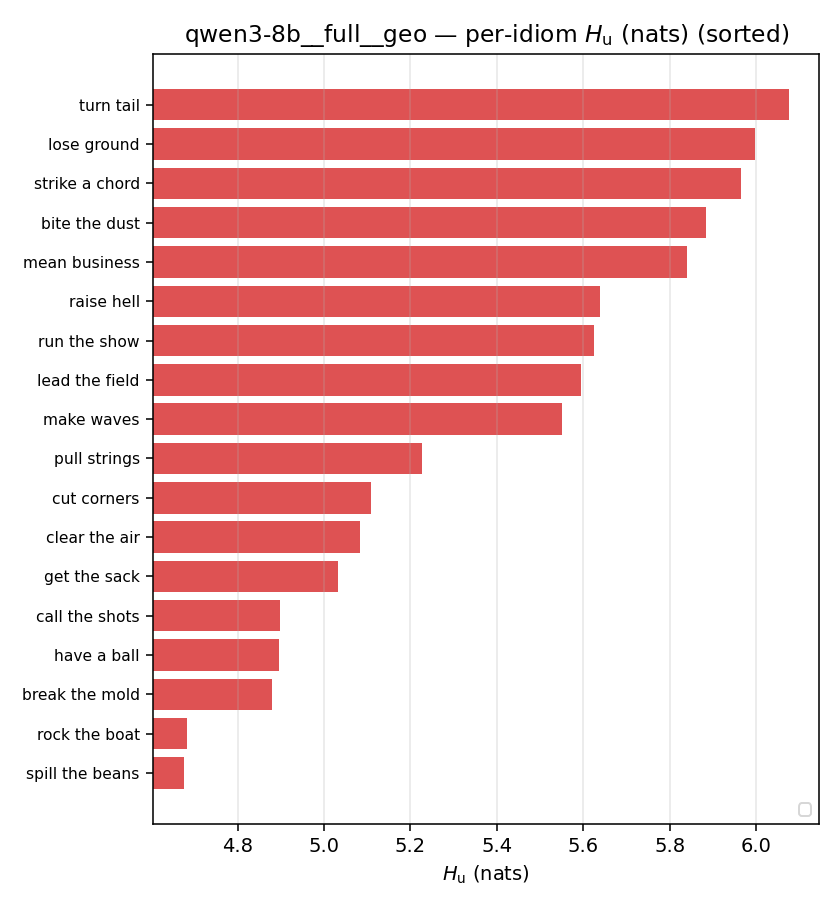 | — (no finite values) | — (no finite values) | 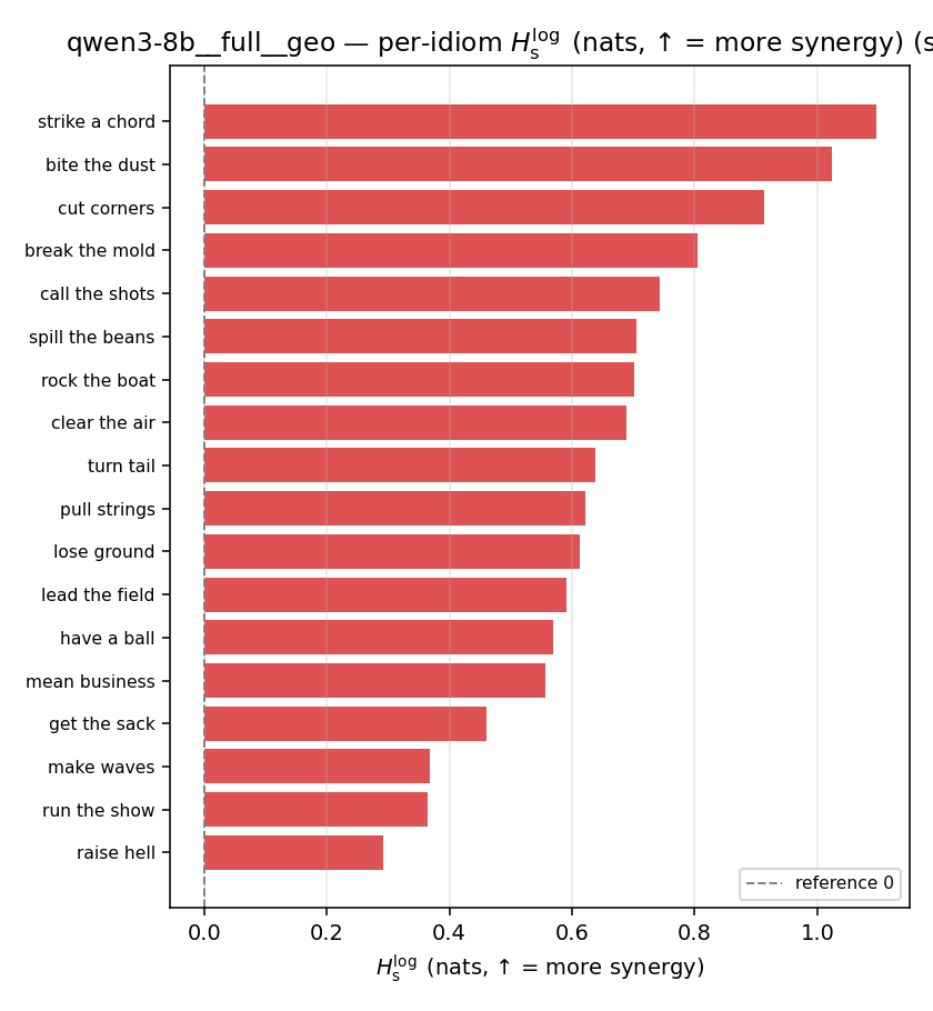 | 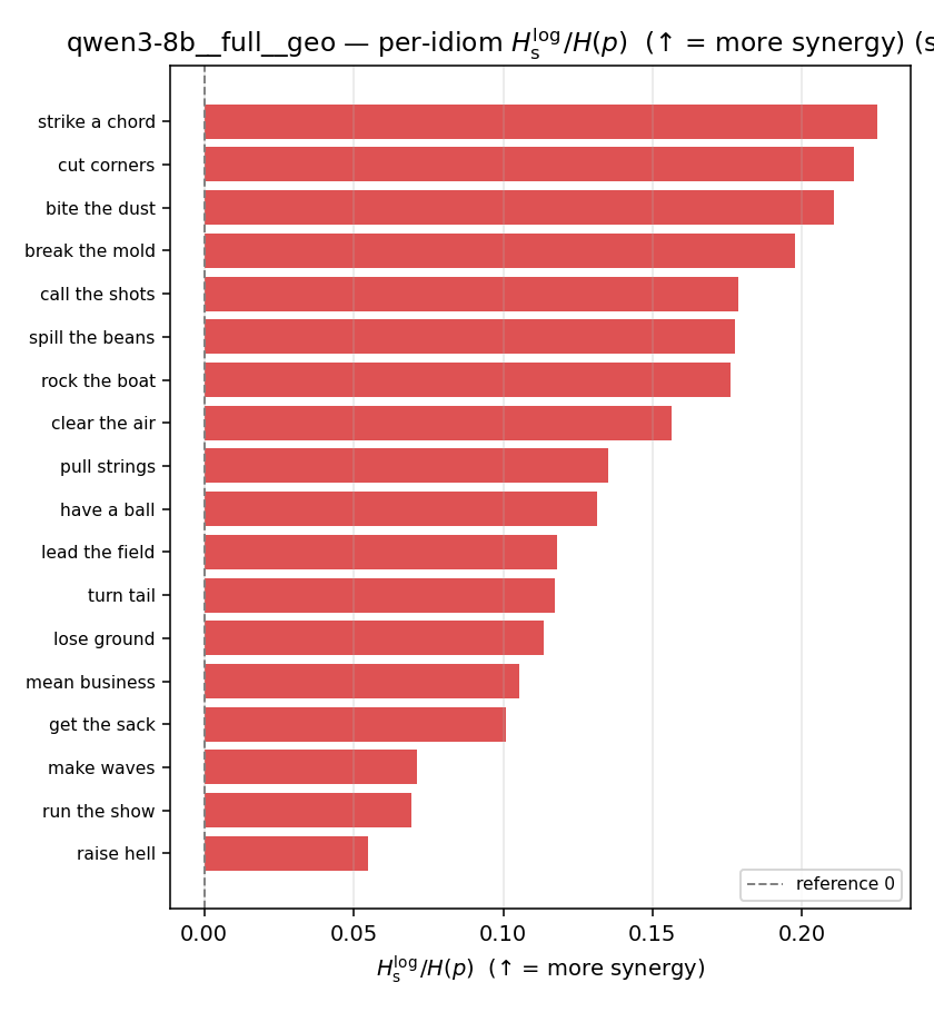 | 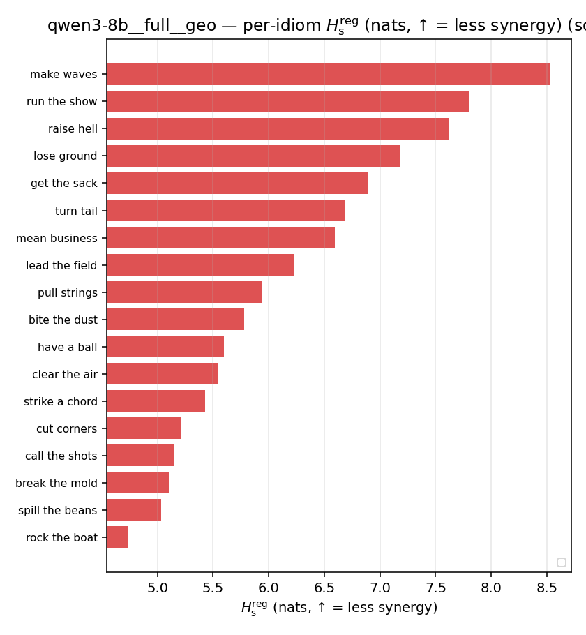 | 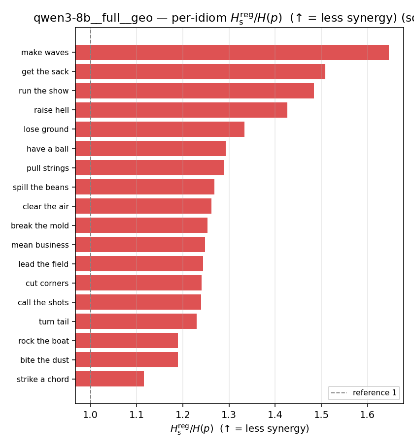 | 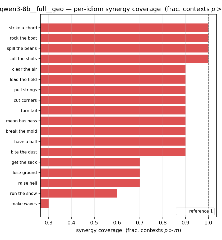 |
qwen3-8b · full · joint qwen3-8b__full__joint
| Ĥu/Ĥ ↑syn | Ĥu | Ĥs ↓syn | Ĥs/Ĥ ↓syn | Ĥslog ↑syn | Ĥslog/Ĥ ↑syn | Ĥsreg ↓syn | Ĥsreg/Ĥ ↓syn | f̂syn ↑syn | |
|---|---|---|---|---|---|---|---|---|---|
| strip (per-phrase) | 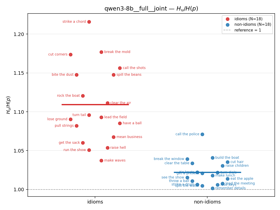 | 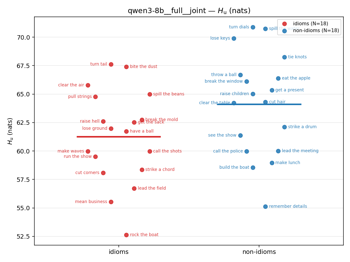 | — (no finite values) | — (no finite values) | 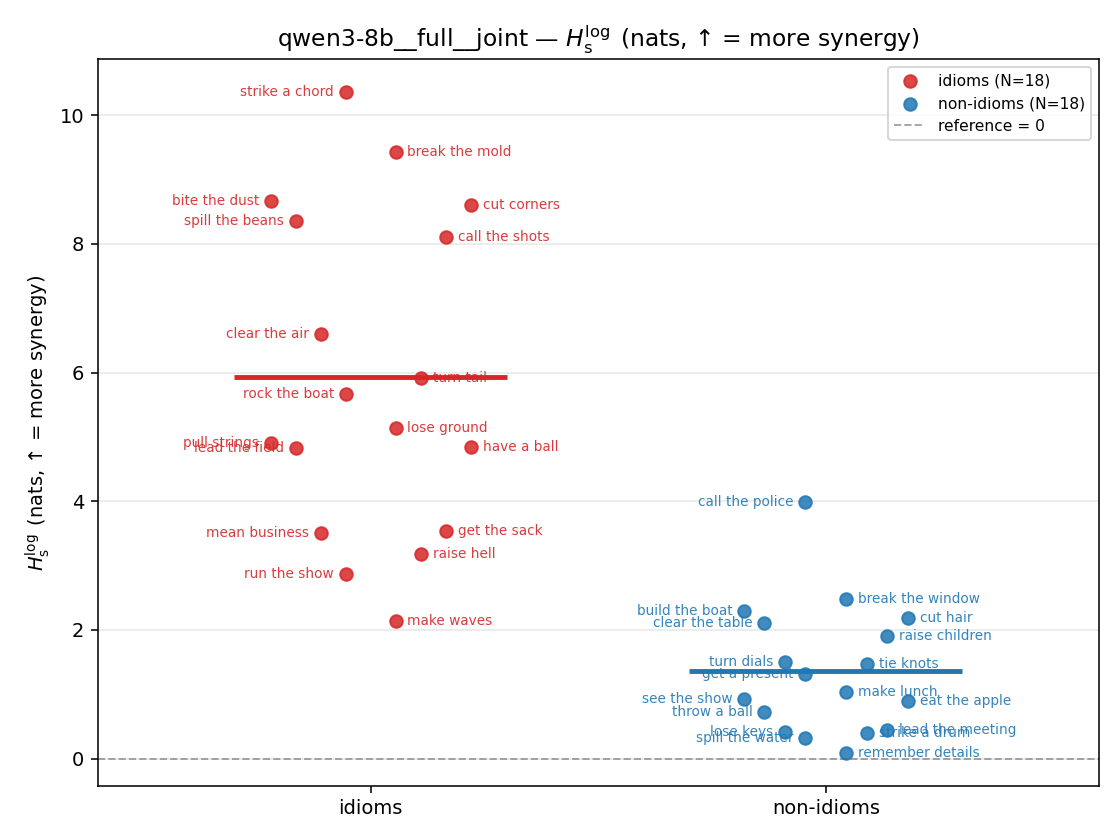 | 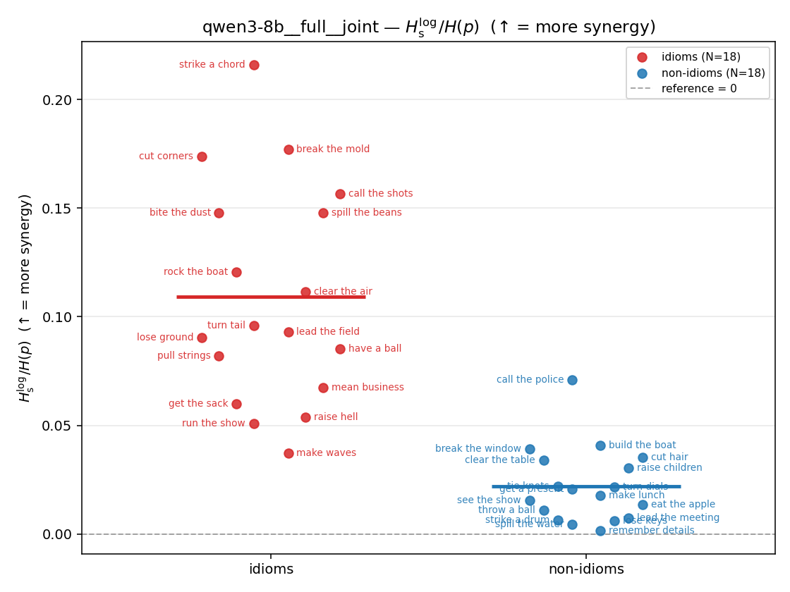 | 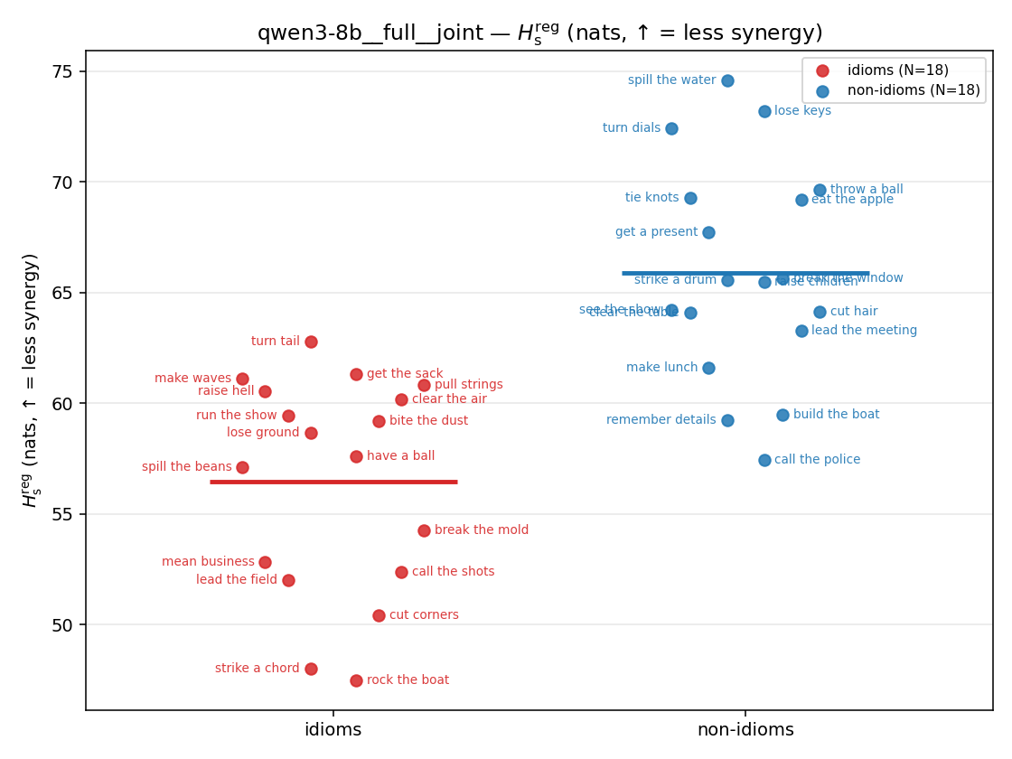 | 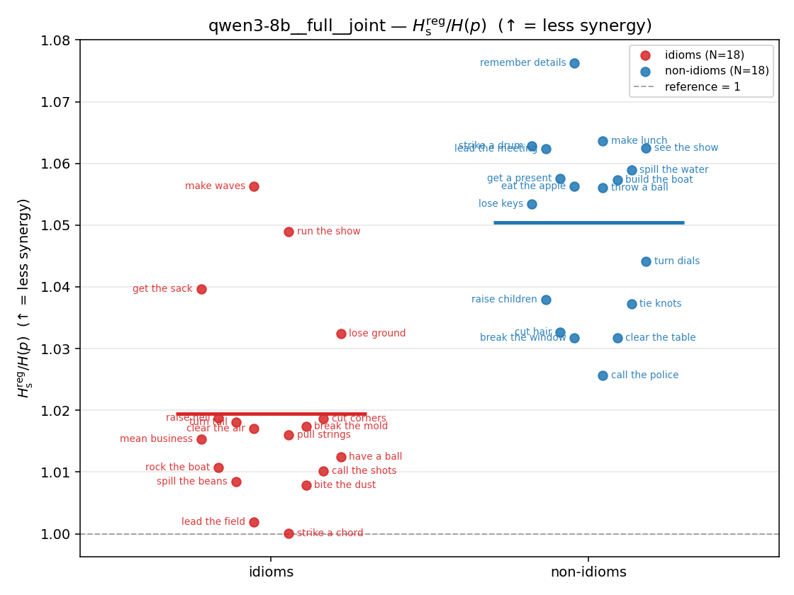 | 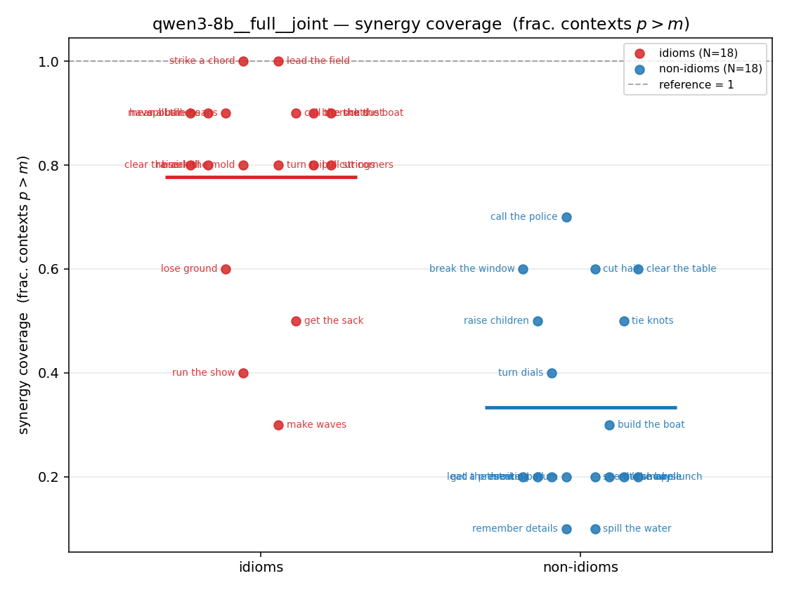 |
| mean ± 95% CI | 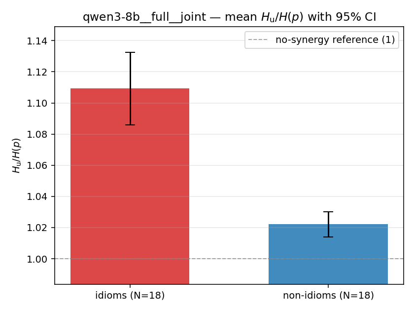 | 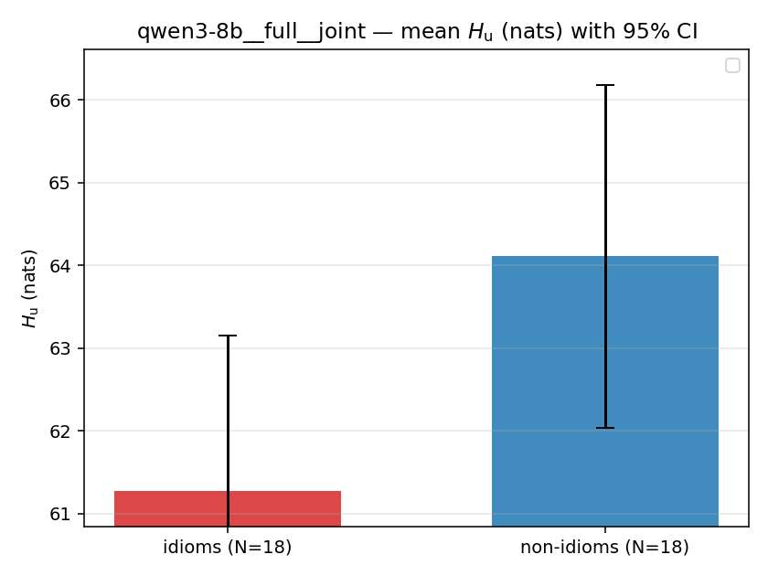 | — (no finite values) | — (no finite values) | 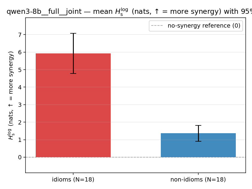 | 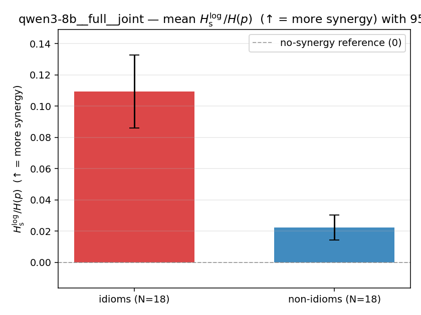 | 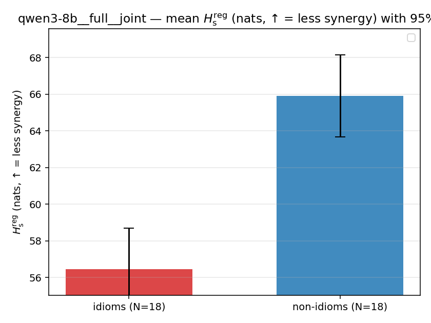 | 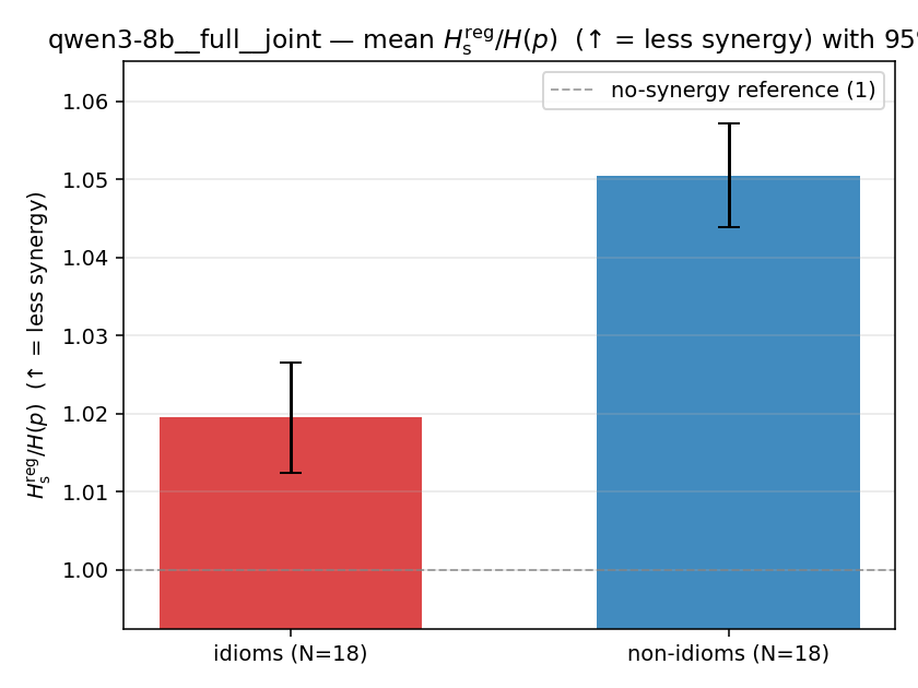 | 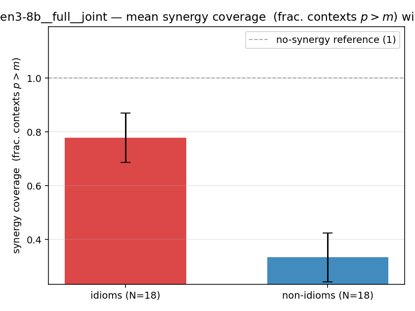 |
| per-idiom (sorted) | 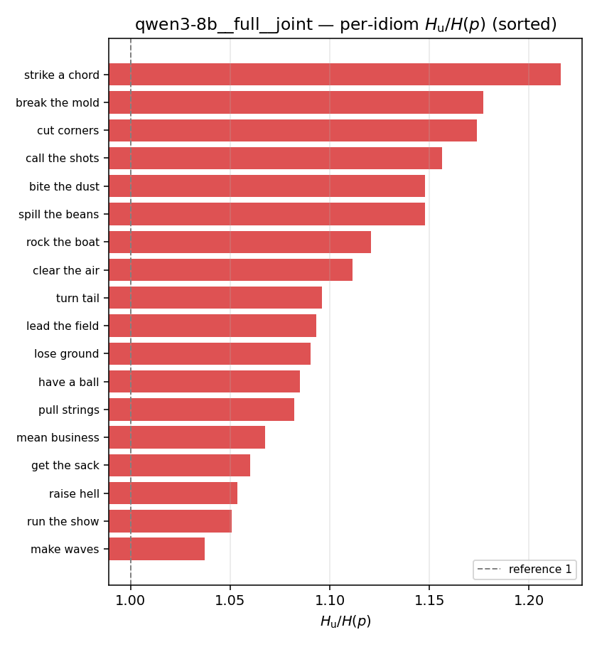 | 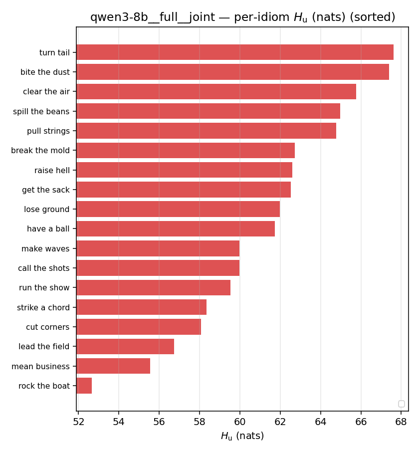 | — (no finite values) | — (no finite values) | 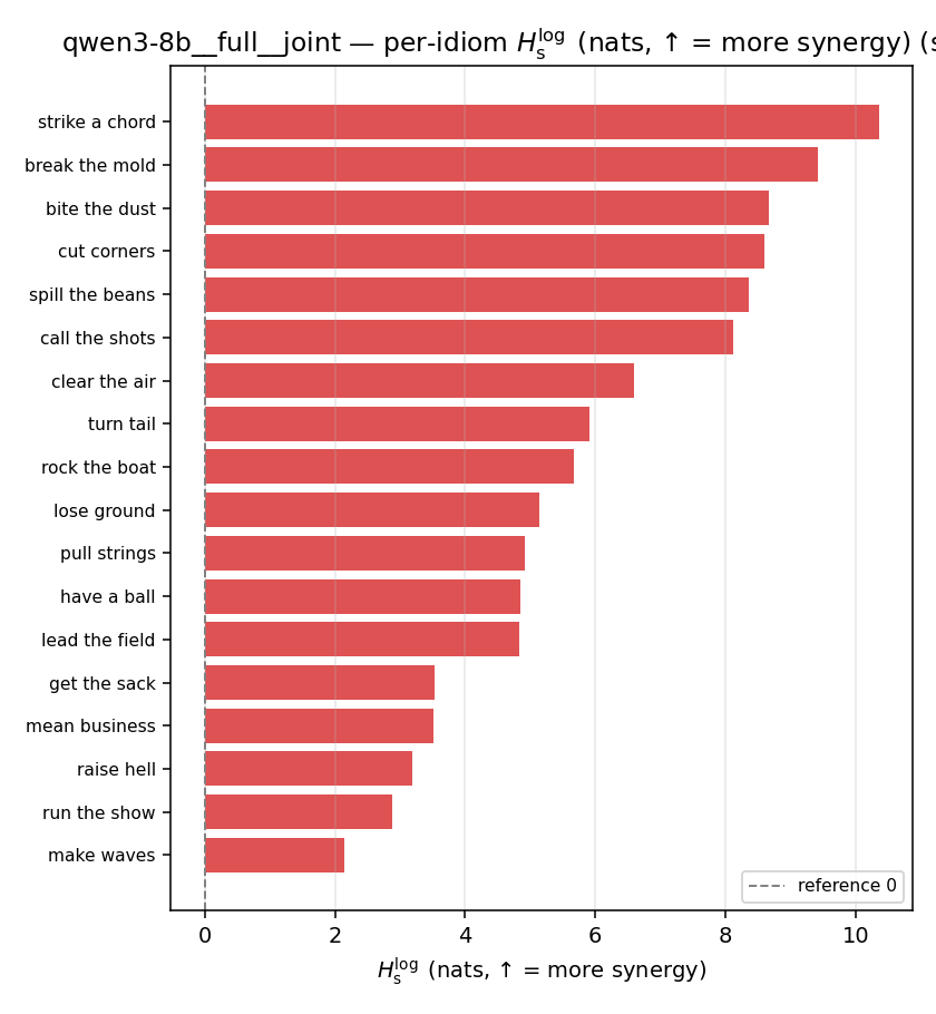 | 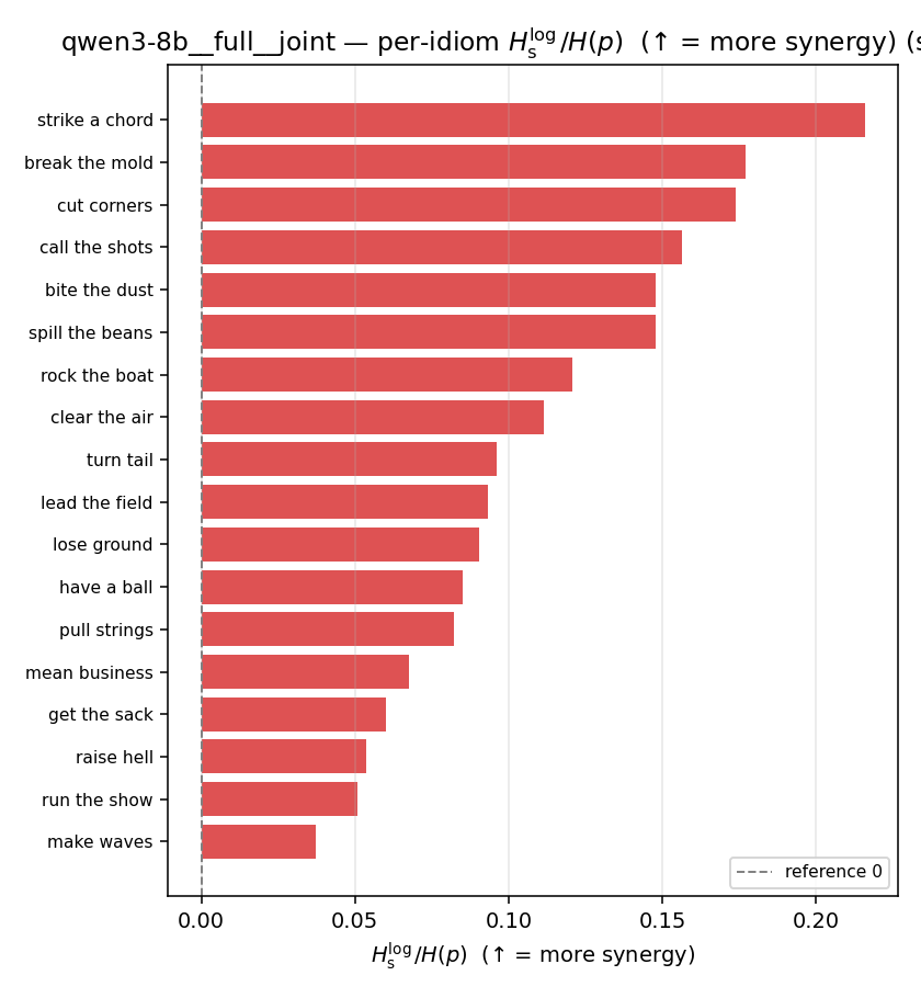 | 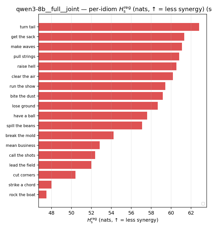 | 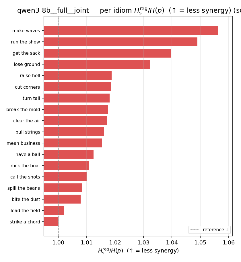 | 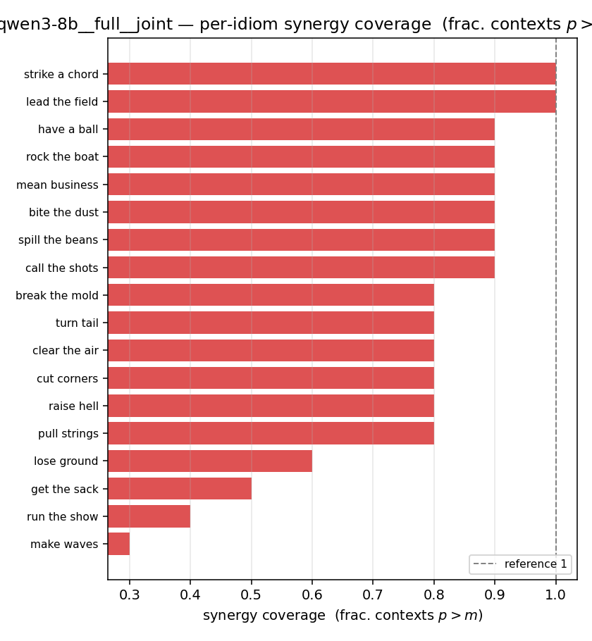 |
llama3.1-8b — per-config figures
3×9 grid of figure-type × metric (↑syn / ↓syn in a header = the metric increases / decreases with synergy; definitions on the entropies page). Tables scroll horizontally; “— (no finite values)” marks Ĥs/ratio_s panels where every phrase was +inf. Click to zoom.
llama3.1-8b · medial · geo llama3.1-8b__medial__geo
| Ĥu/Ĥ ↑syn | Ĥu | Ĥs ↓syn | Ĥs/Ĥ ↓syn | Ĥslog ↑syn | Ĥslog/Ĥ ↑syn | Ĥsreg ↓syn | Ĥsreg/Ĥ ↓syn | f̂syn ↑syn | |
|---|---|---|---|---|---|---|---|---|---|
| strip (per-phrase) | 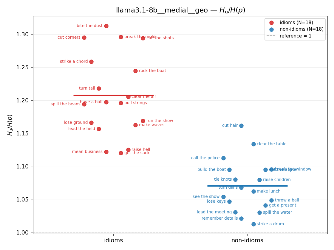 | 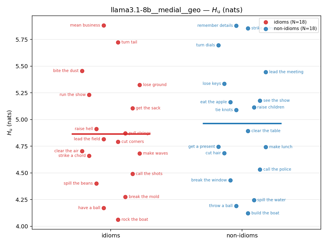 | 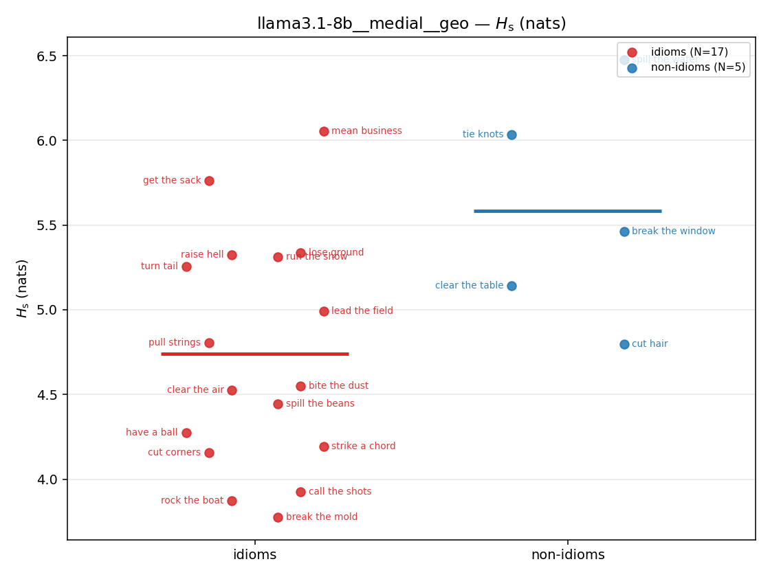 | 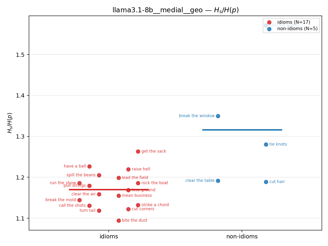 | 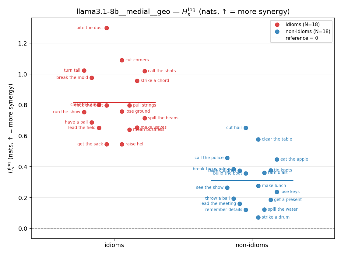 | 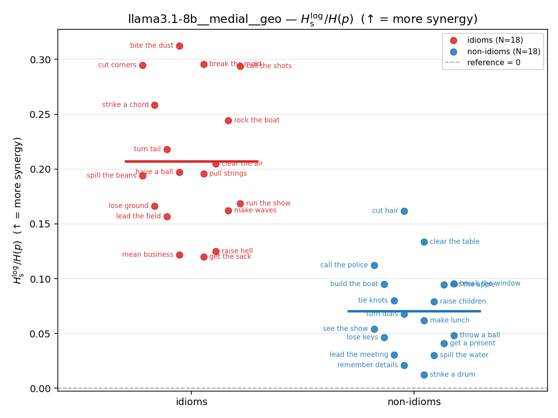 | 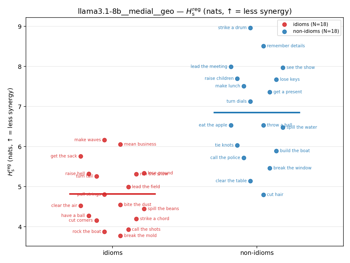 | 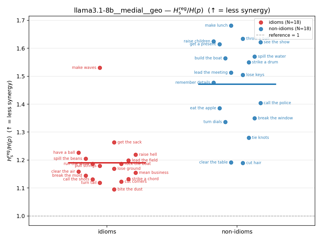 | 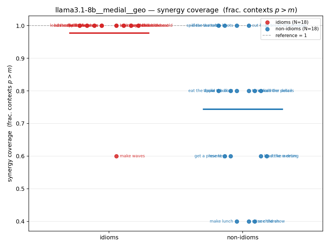 |
| mean ± 95% CI | 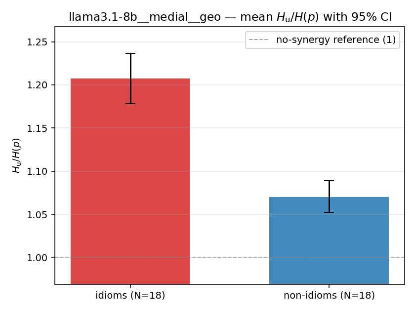 | 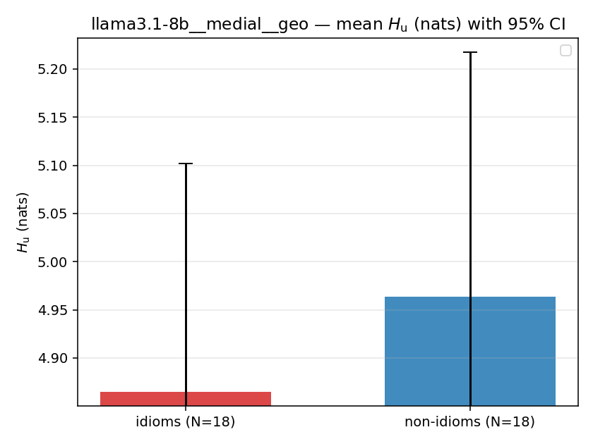 | 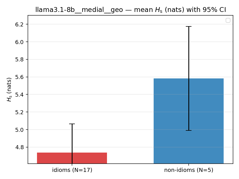 | 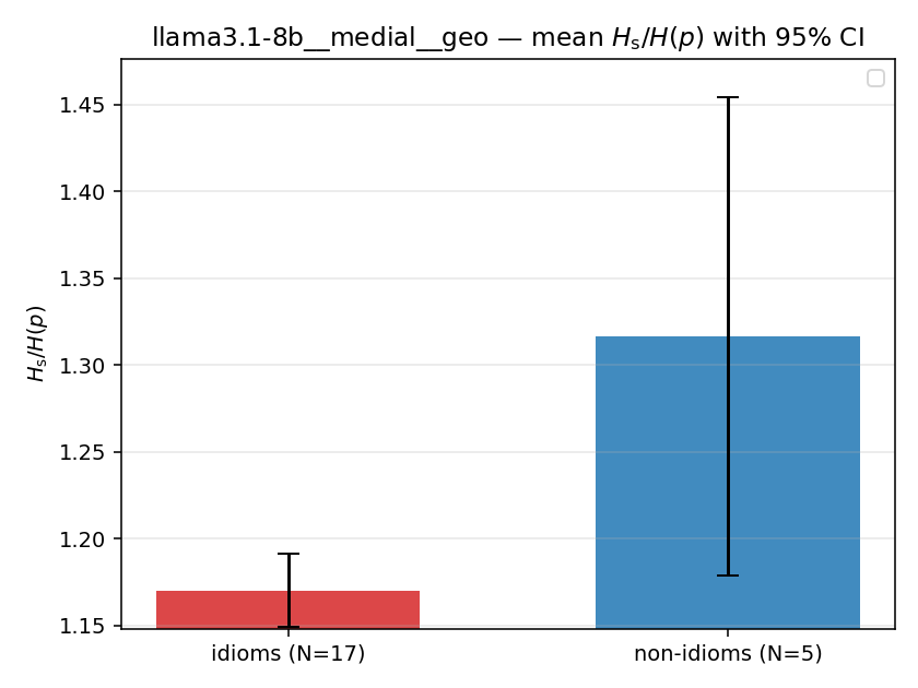 | 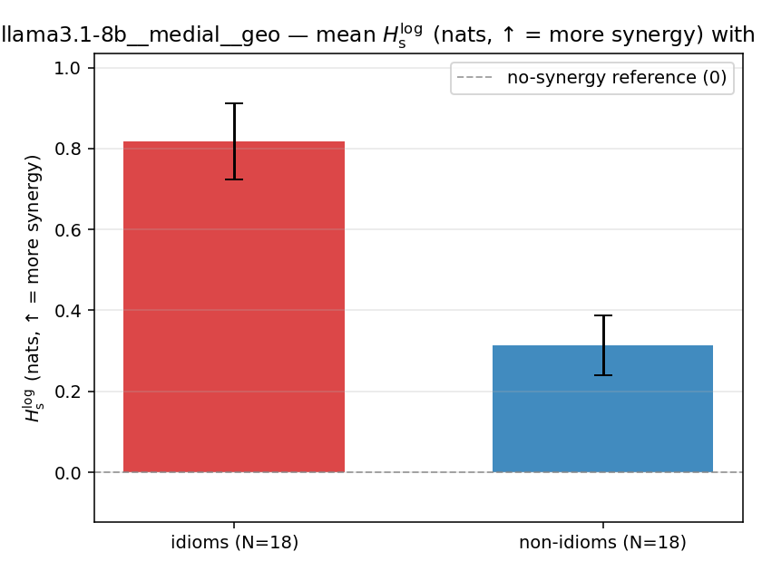 | 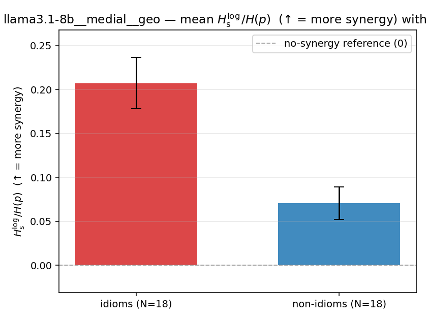 | 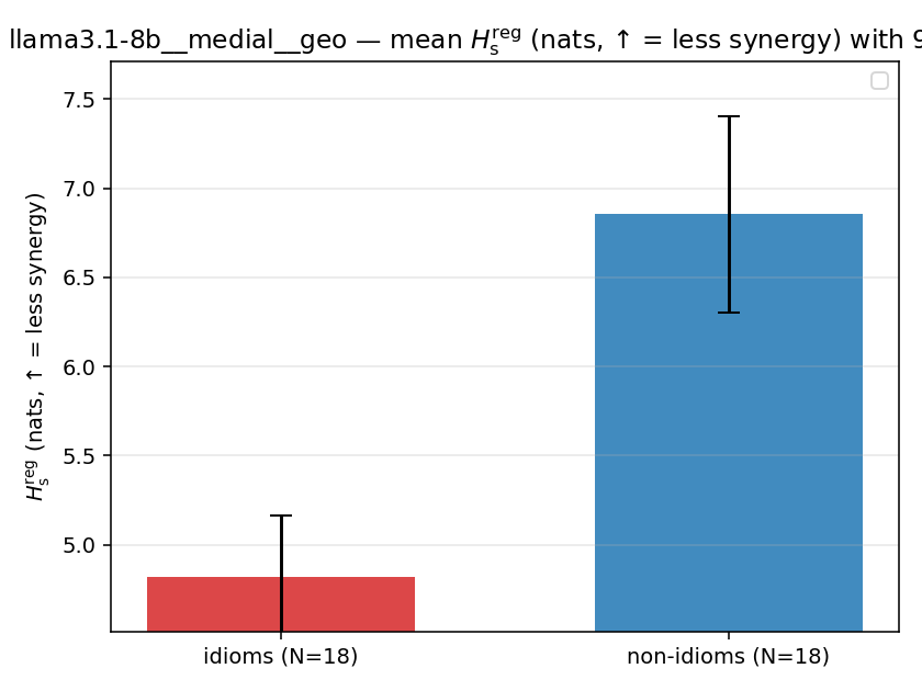 | 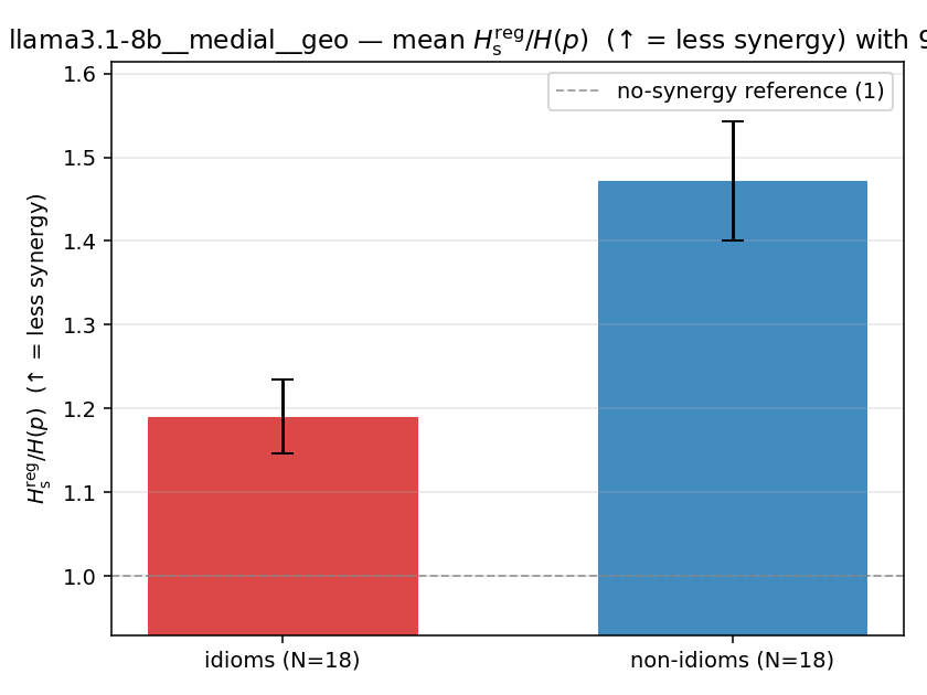 | 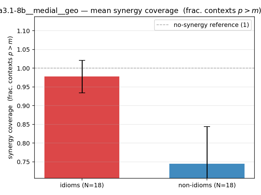 |
| per-idiom (sorted) | 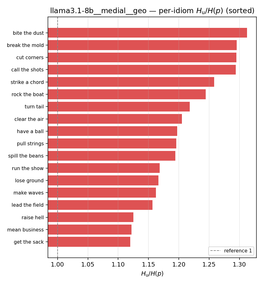 | 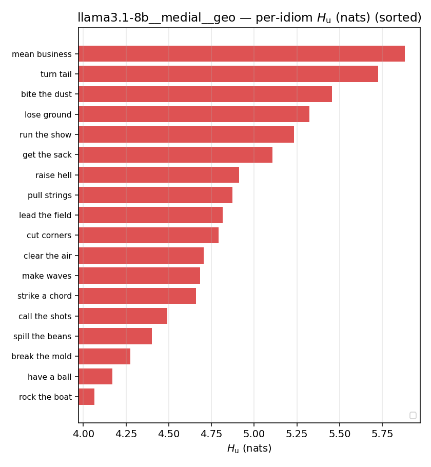 | 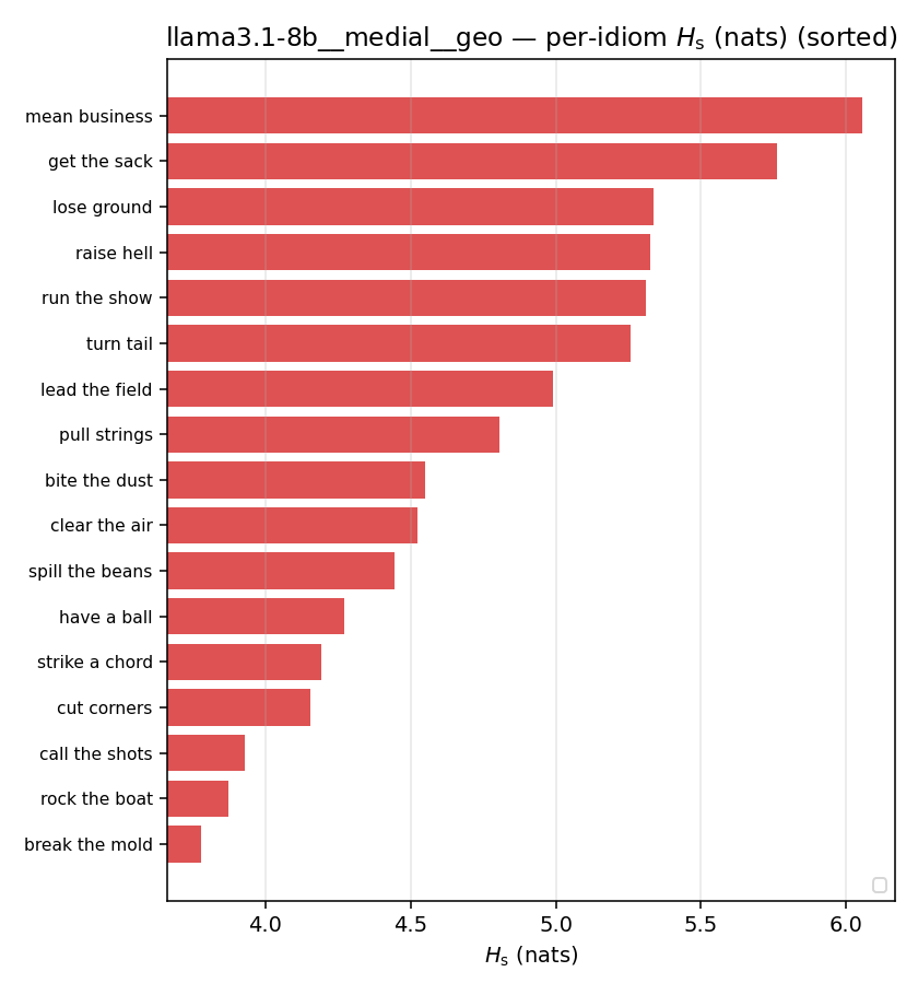 | 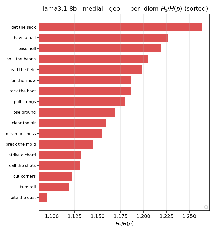 | 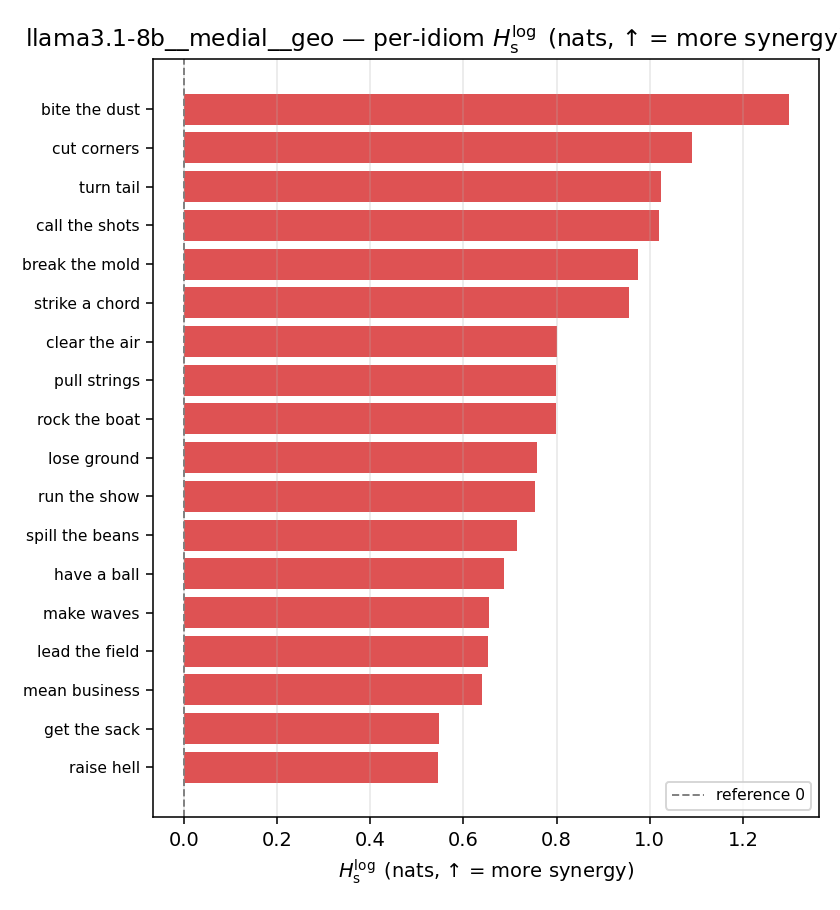 | 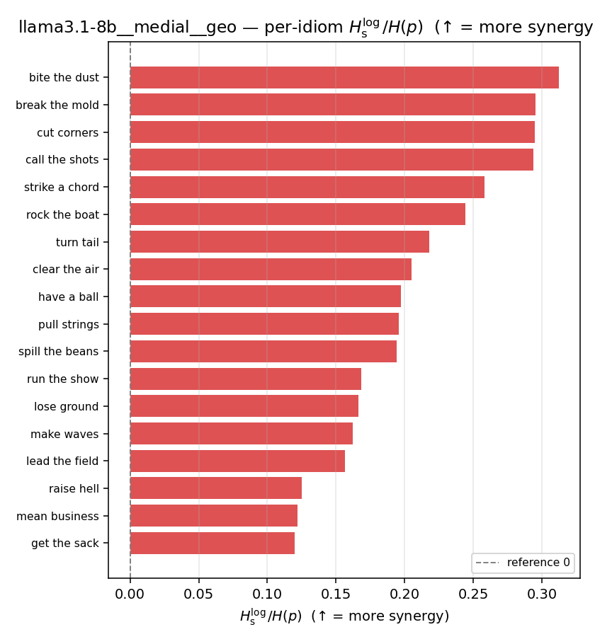 | 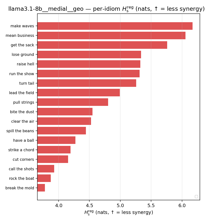 | 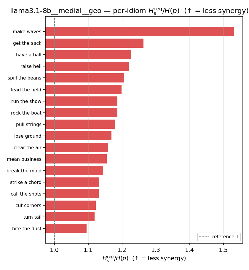 | 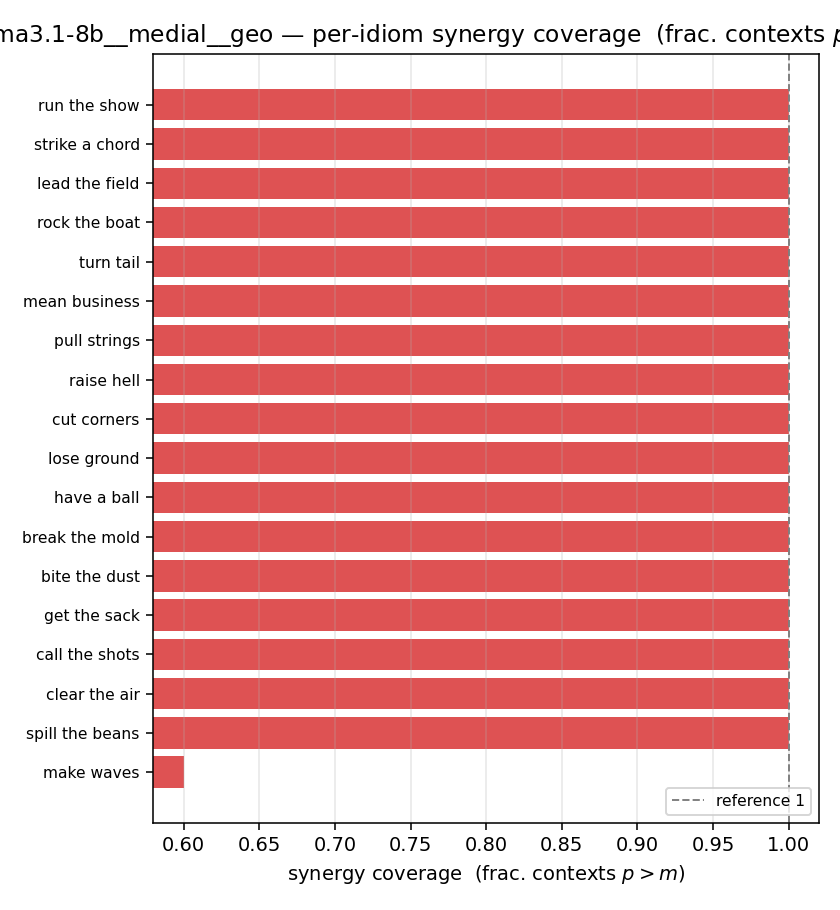 |
llama3.1-8b · medial · joint llama3.1-8b__medial__joint
| Ĥu/Ĥ ↑syn | Ĥu | Ĥs ↓syn | Ĥs/Ĥ ↓syn | Ĥslog ↑syn | Ĥslog/Ĥ ↑syn | Ĥsreg ↓syn | Ĥsreg/Ĥ ↓syn | f̂syn ↑syn | |
|---|---|---|---|---|---|---|---|---|---|
| strip (per-phrase) | 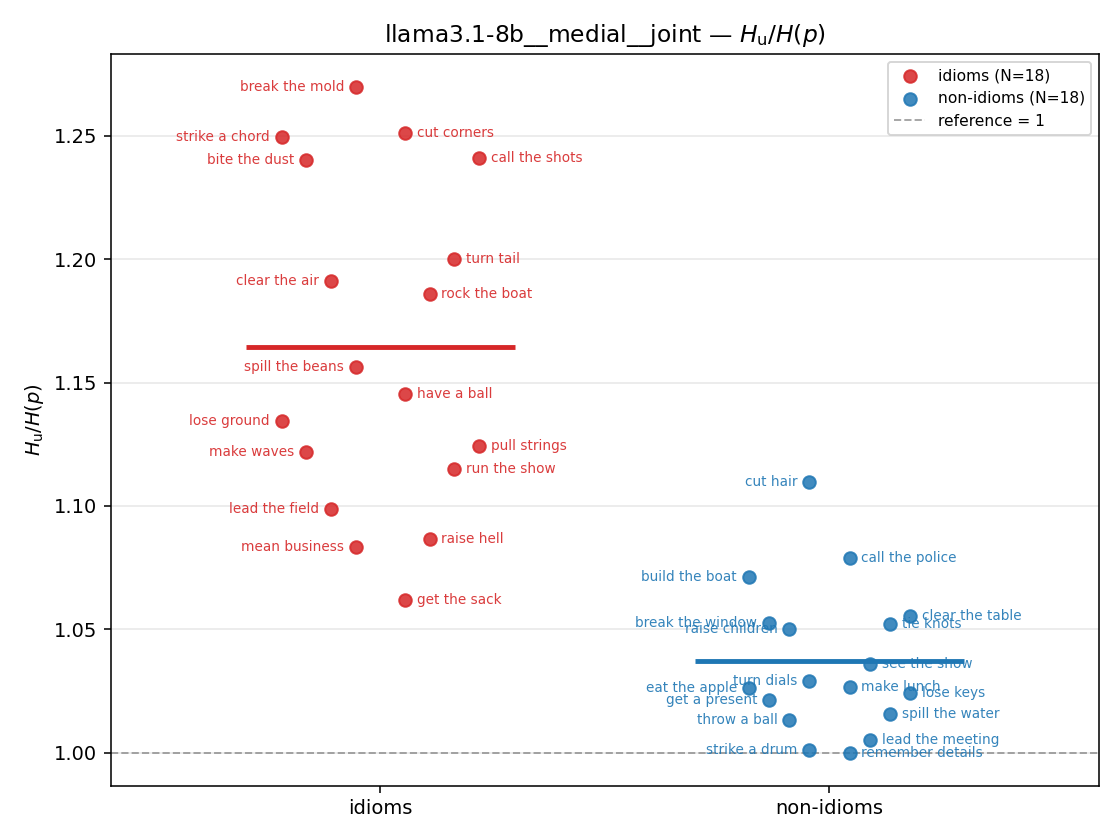 | 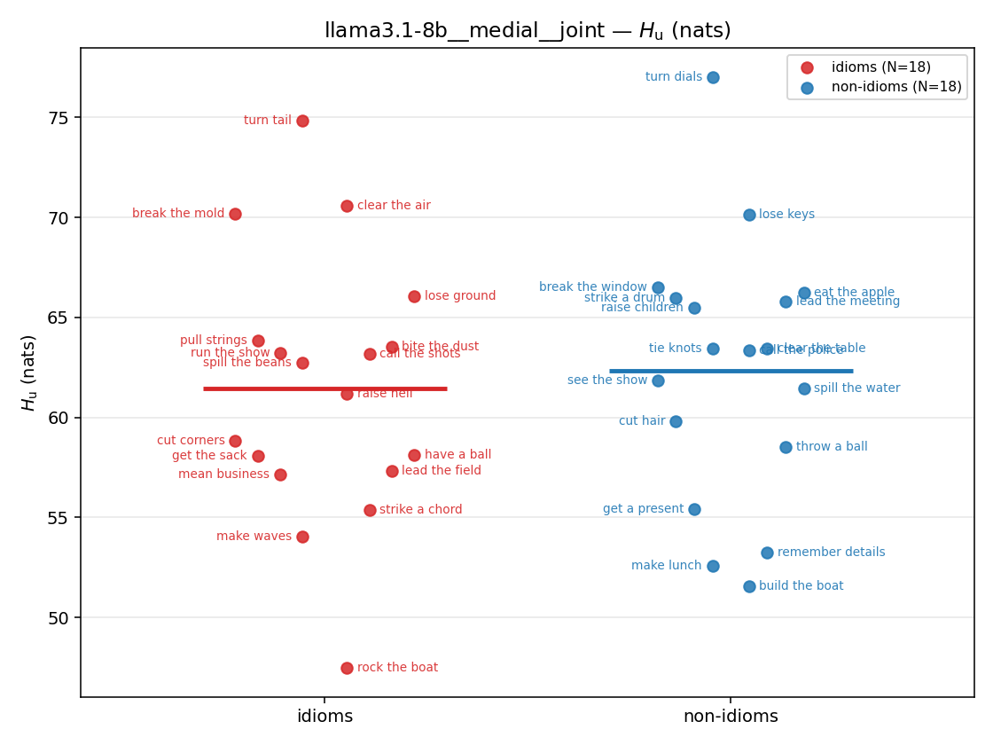 | 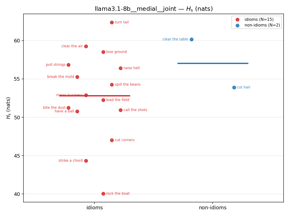 | 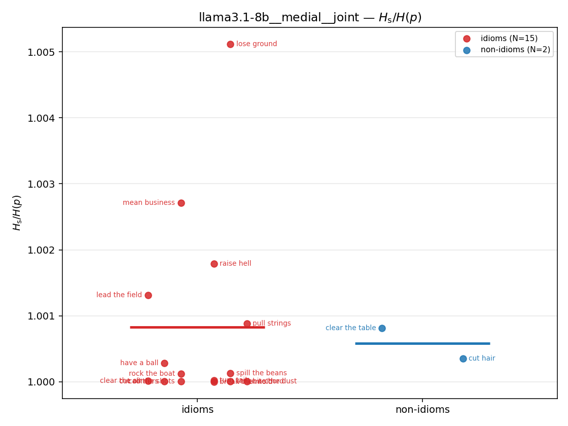 | 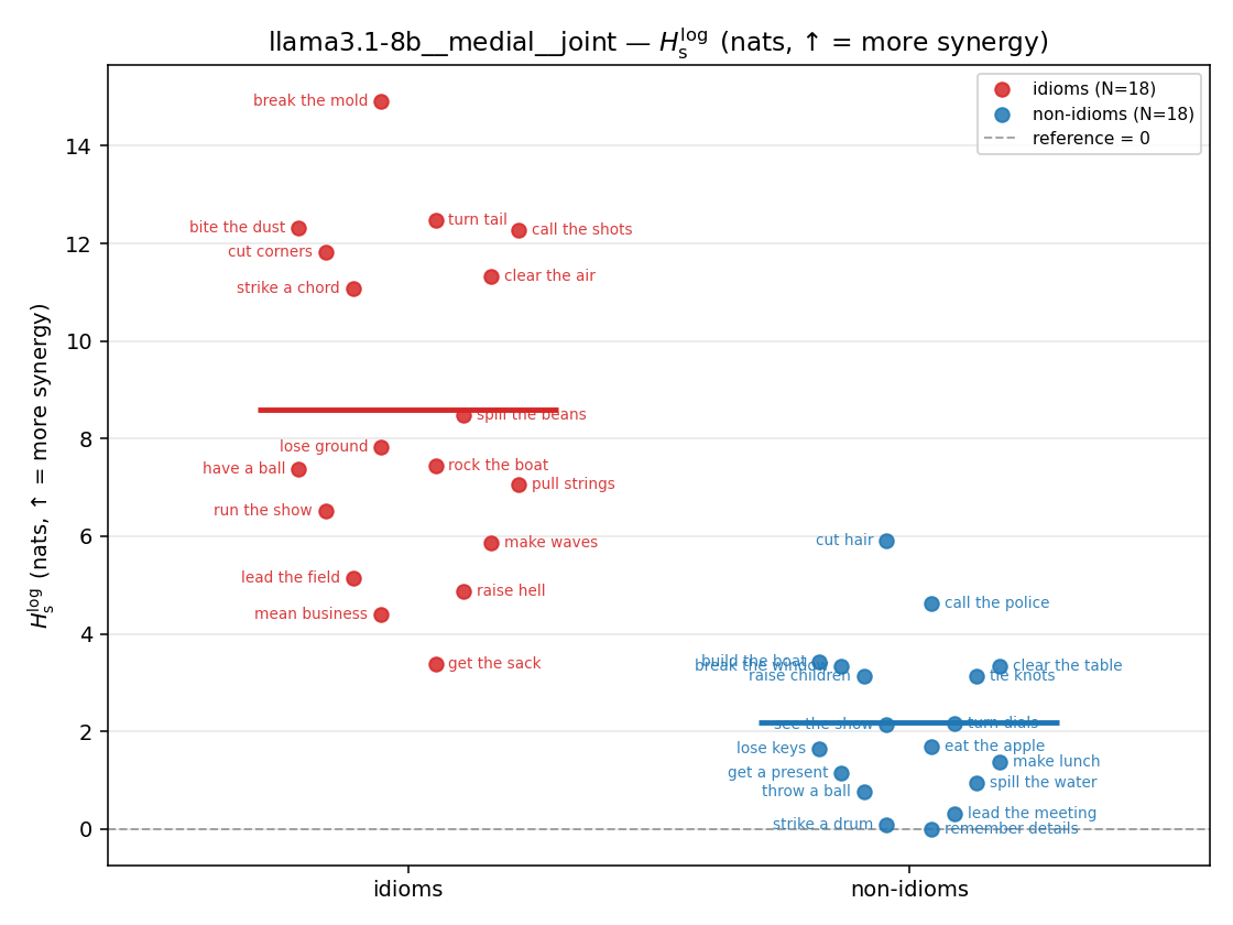 | 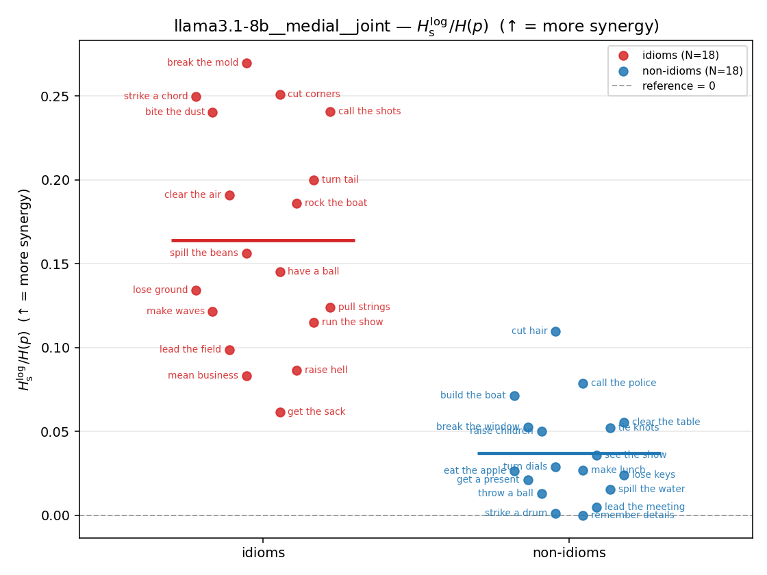 | 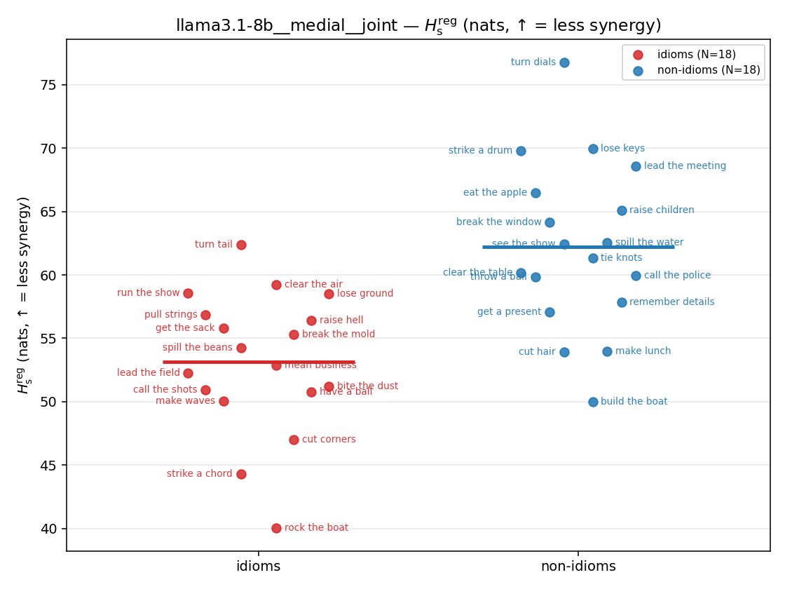 | 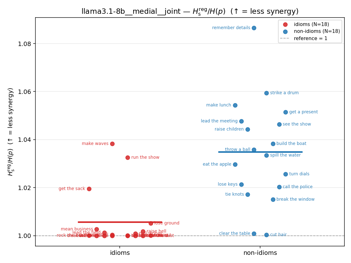 | 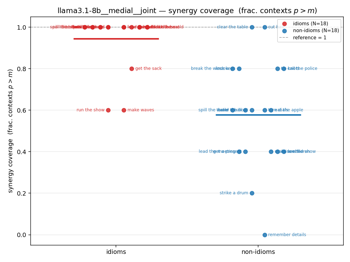 |
| mean ± 95% CI | 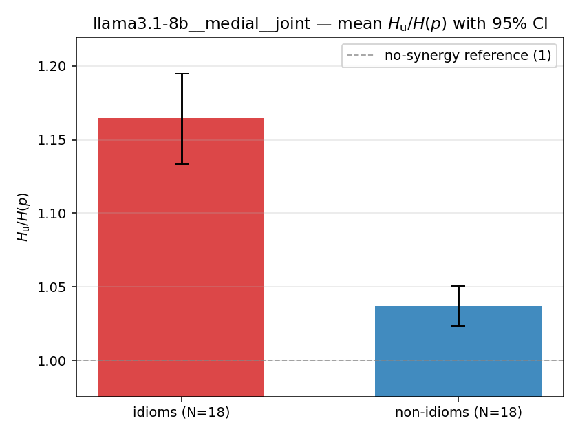 | 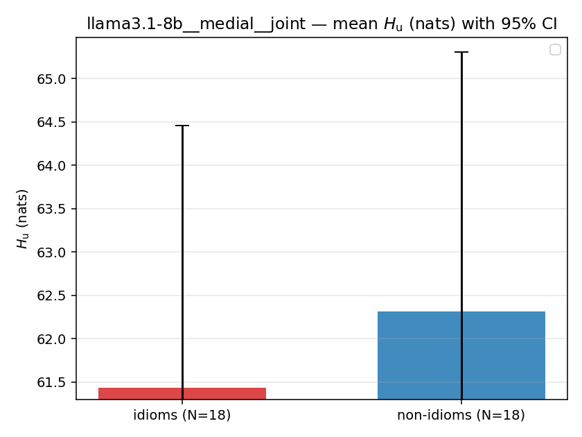 | 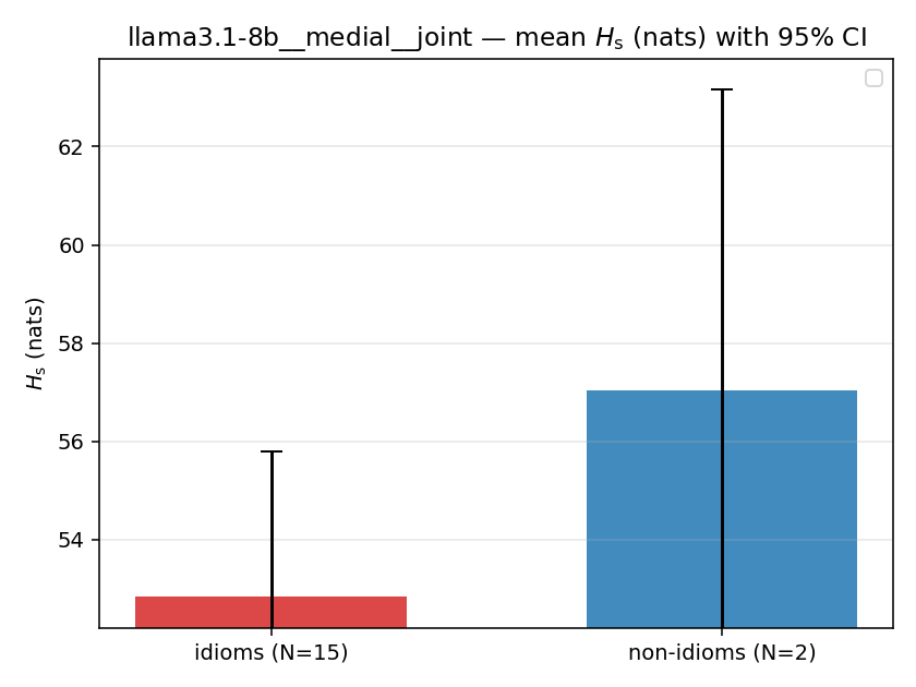 | 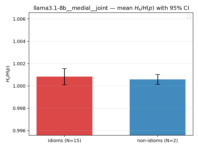 | 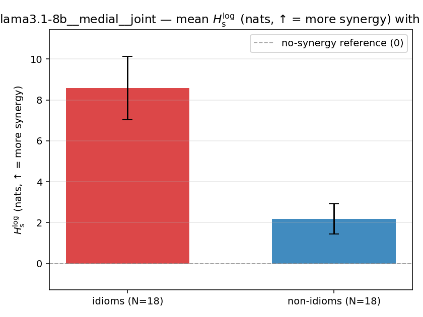 | 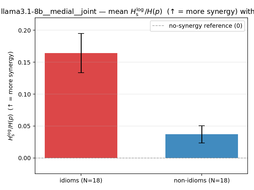 | 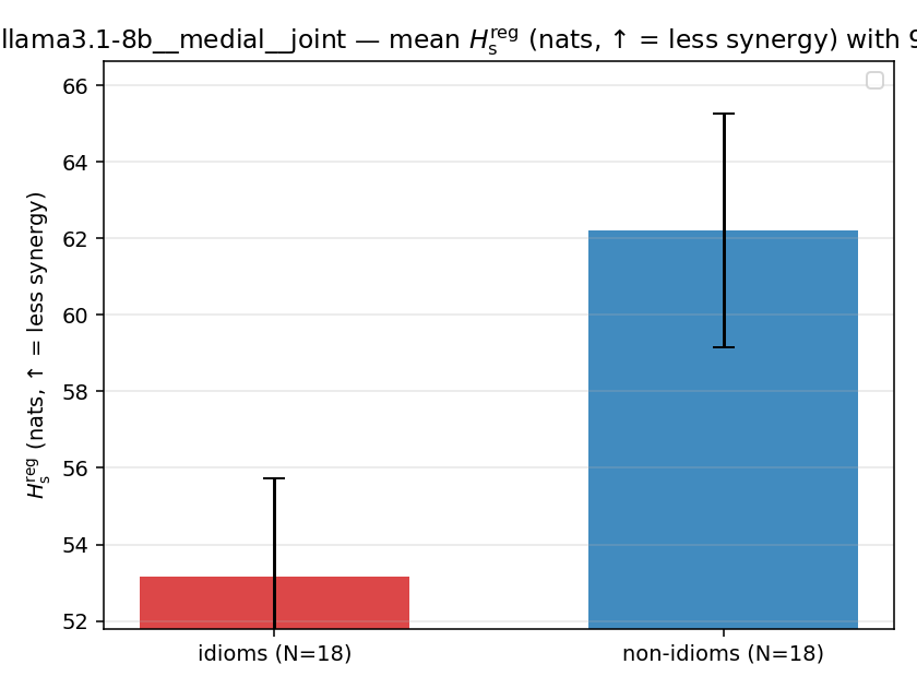 | 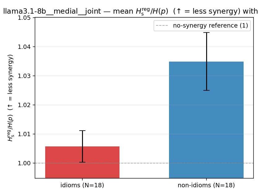 | 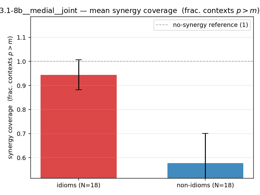 |
| per-idiom (sorted) | 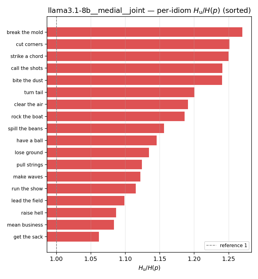 | 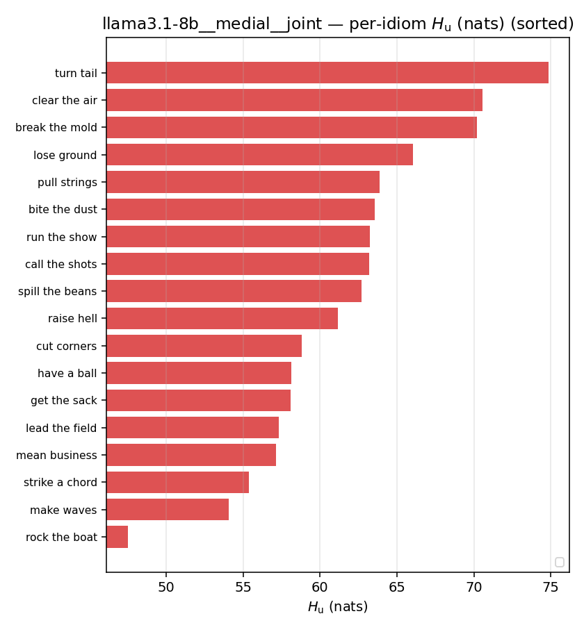 | 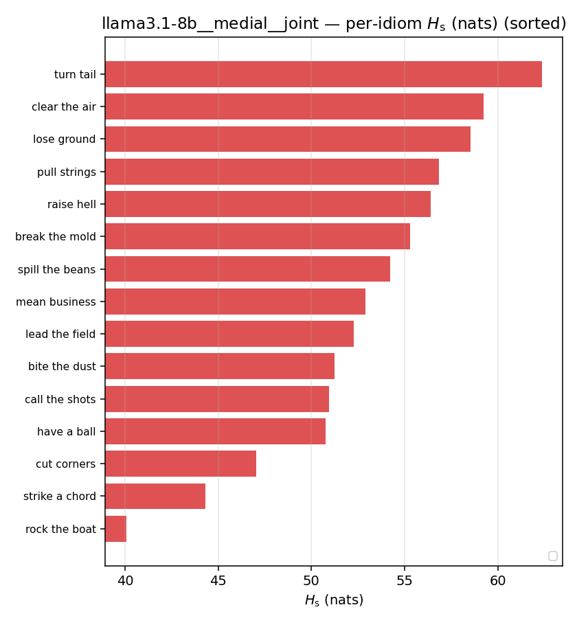 | 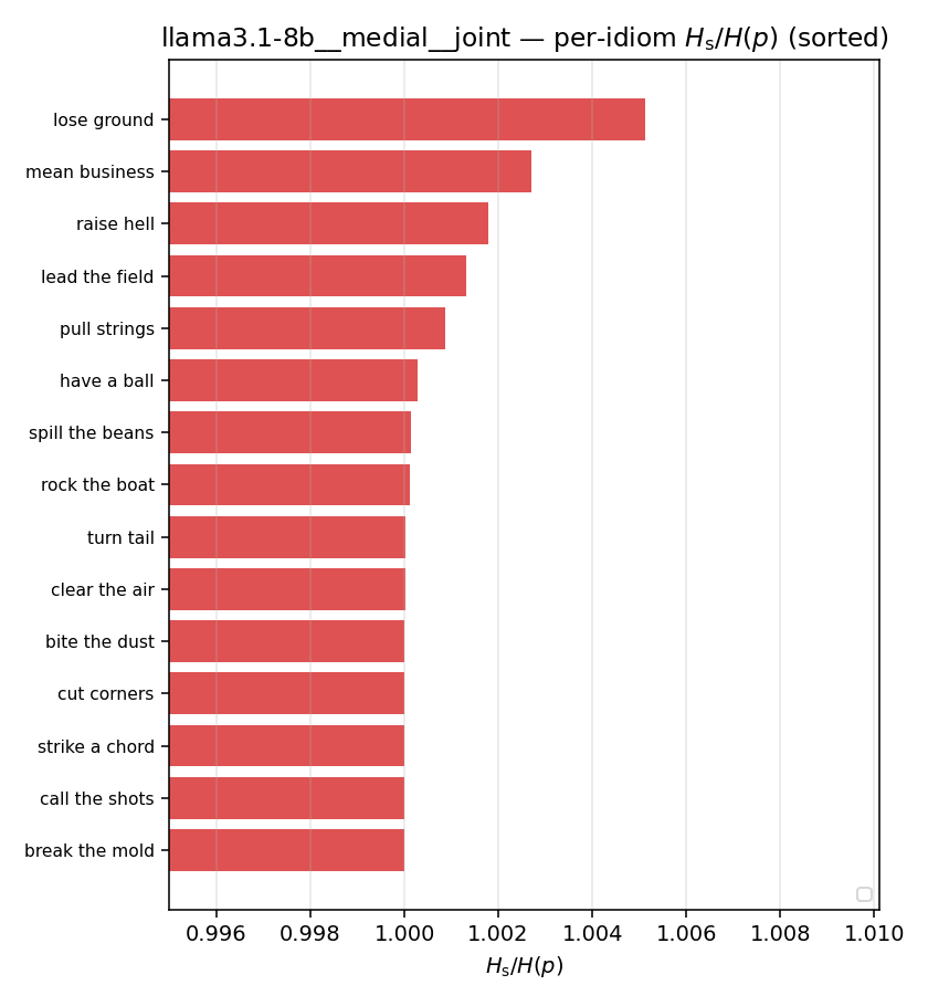 | 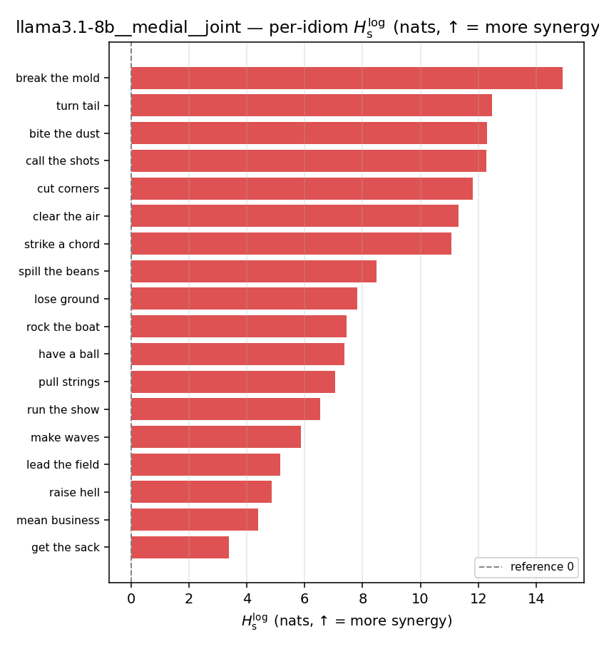 | 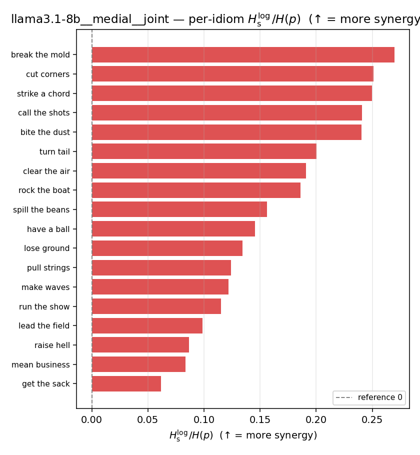 | 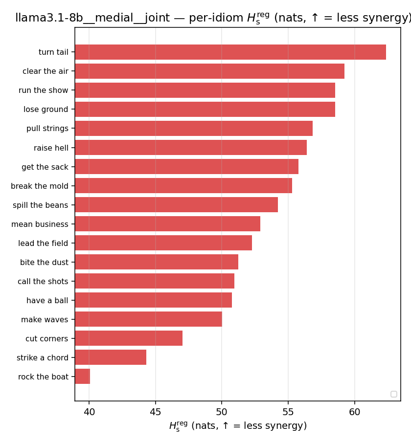 | 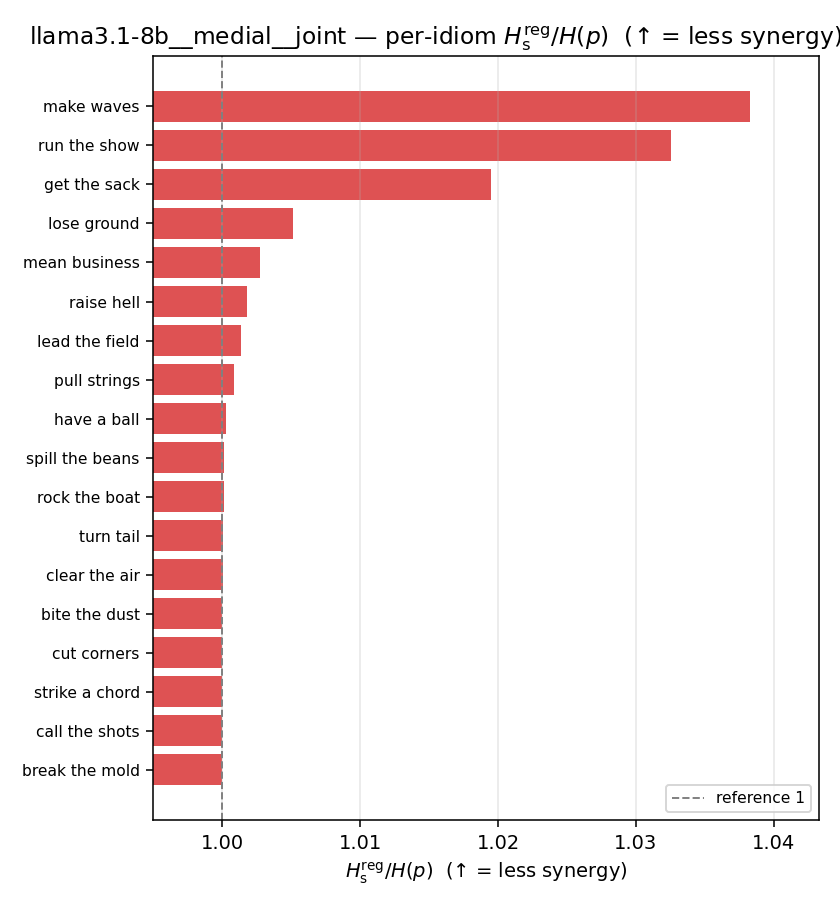 | 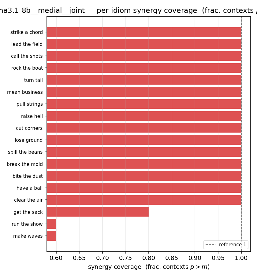 |
llama3.1-8b · full · geo llama3.1-8b__full__geo
| Ĥu/Ĥ ↑syn | Ĥu | Ĥs ↓syn | Ĥs/Ĥ ↓syn | Ĥslog ↑syn | Ĥslog/Ĥ ↑syn | Ĥsreg ↓syn | Ĥsreg/Ĥ ↓syn | f̂syn ↑syn | |
|---|---|---|---|---|---|---|---|---|---|
| strip (per-phrase) | 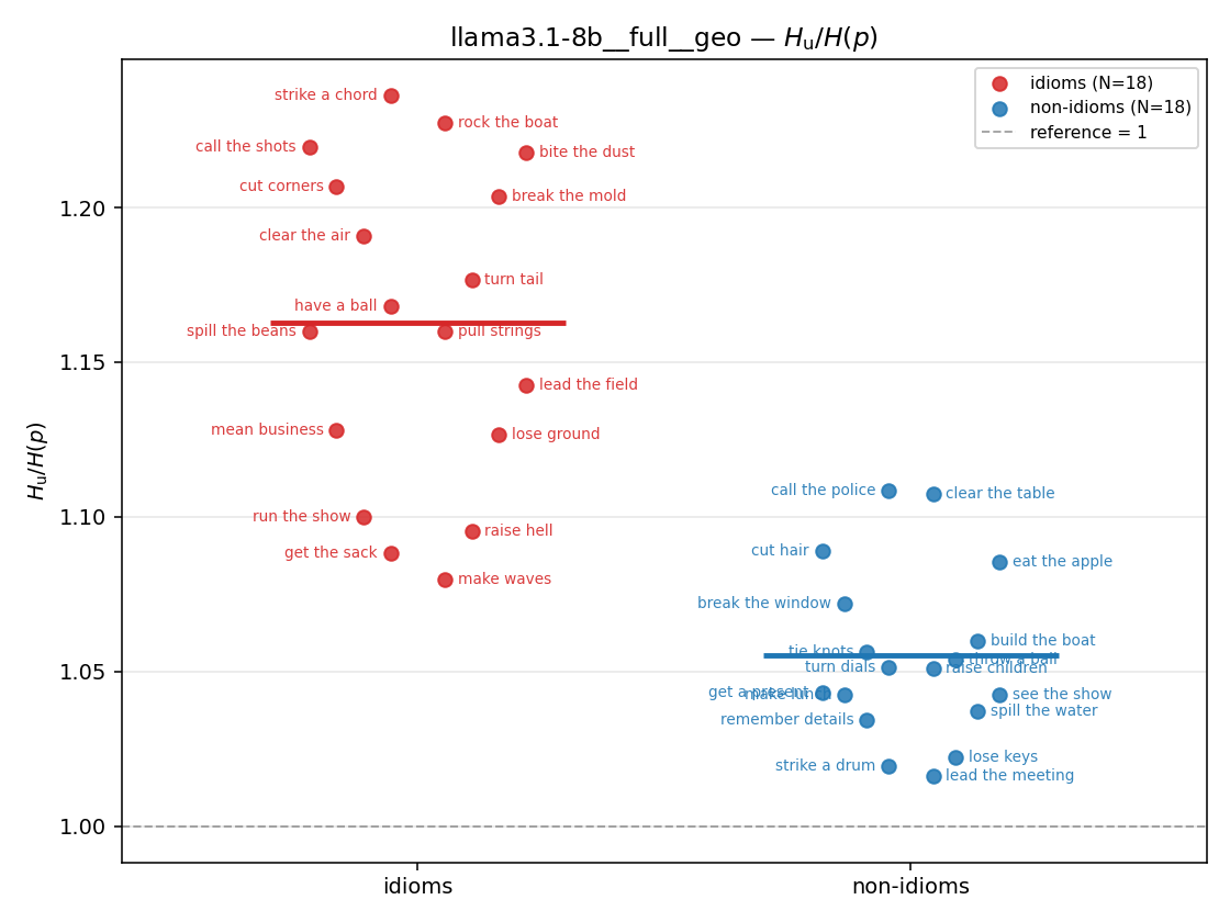 | 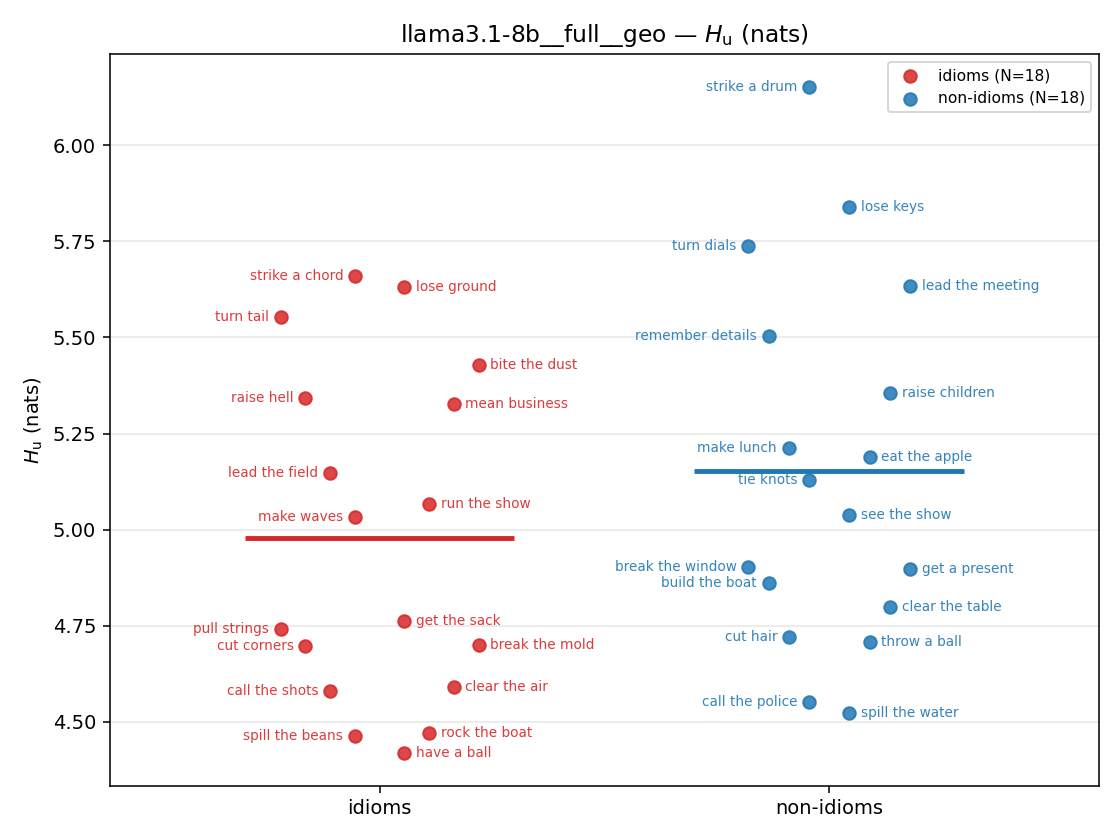 | 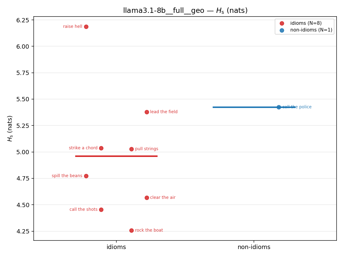 | 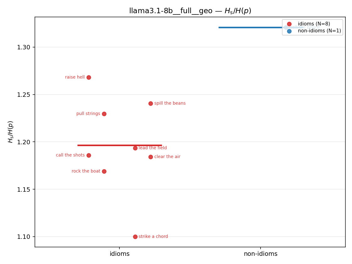 | 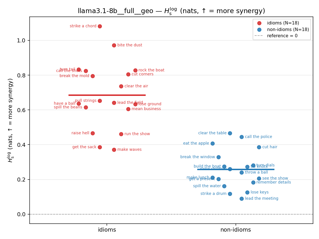 | 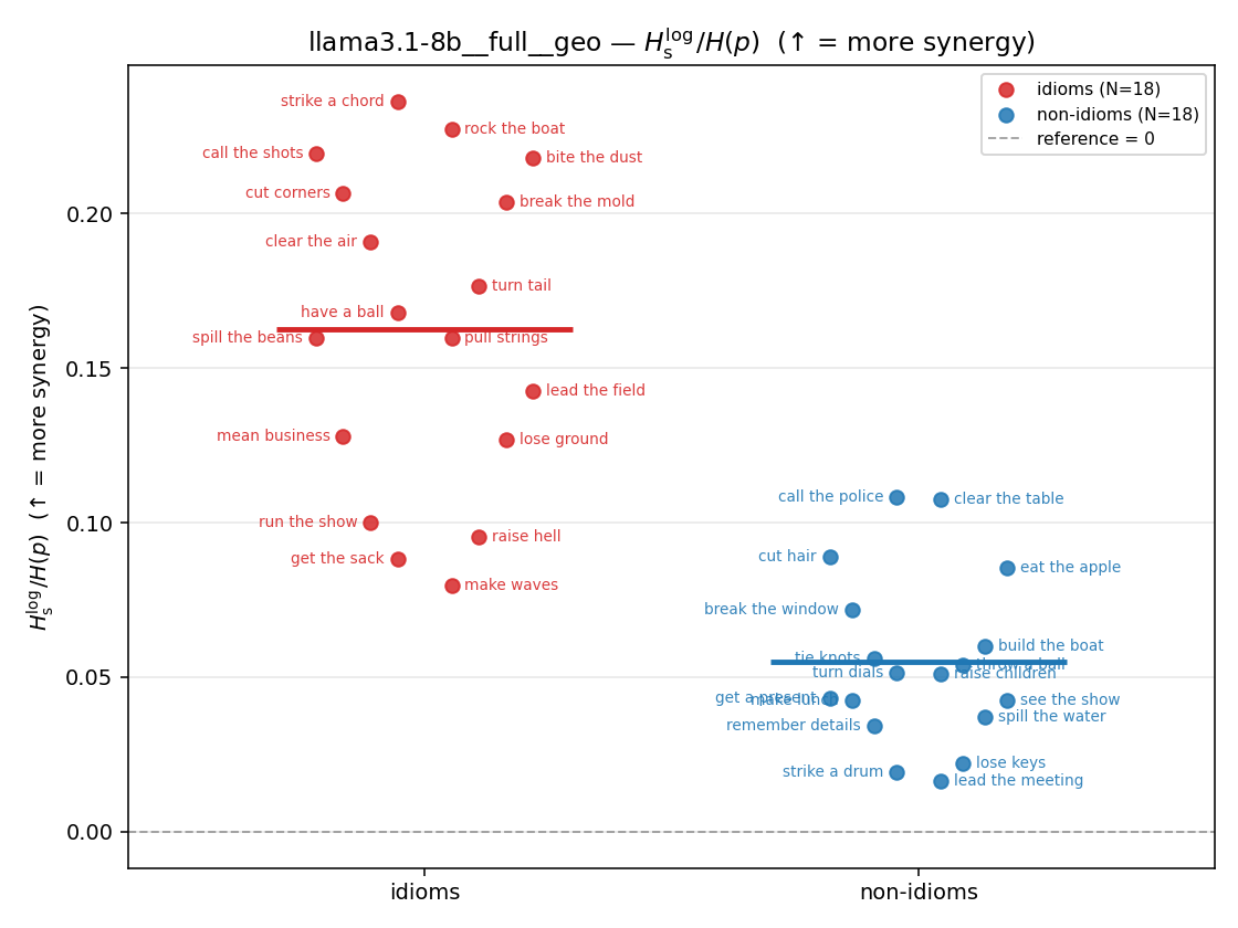 | 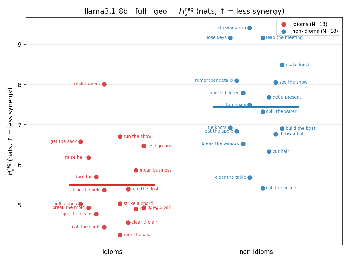 | 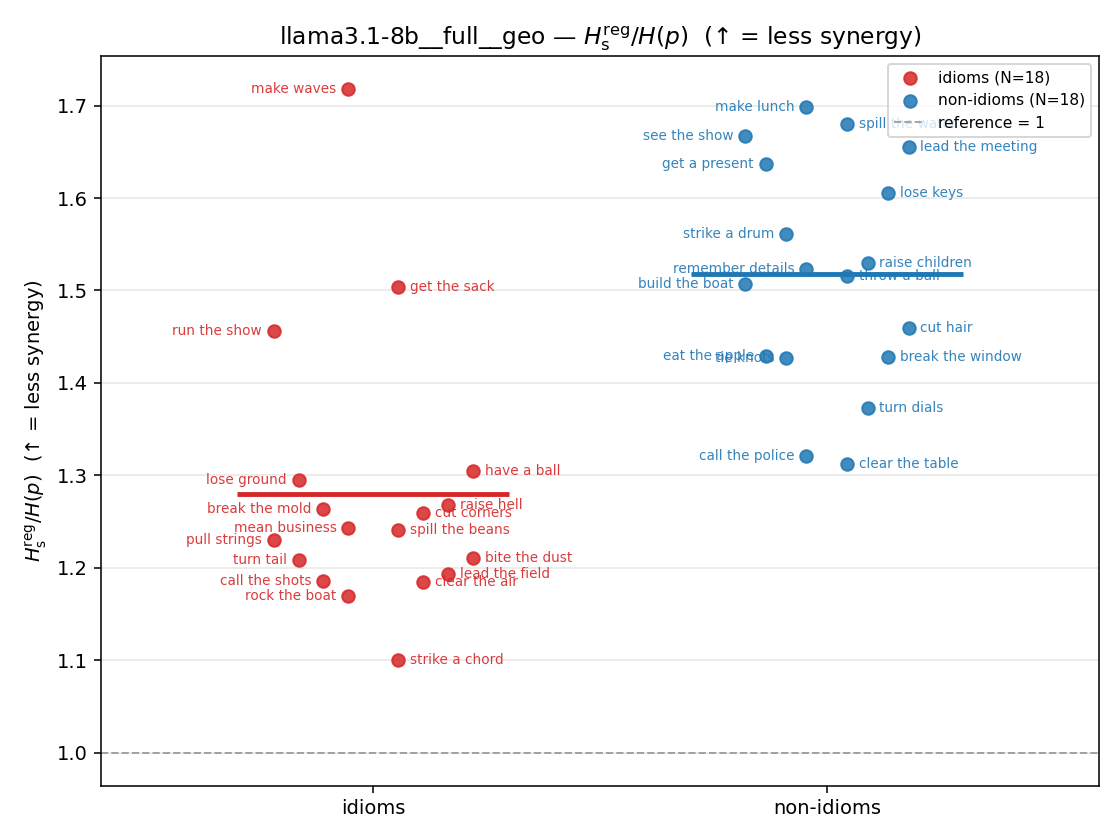 | 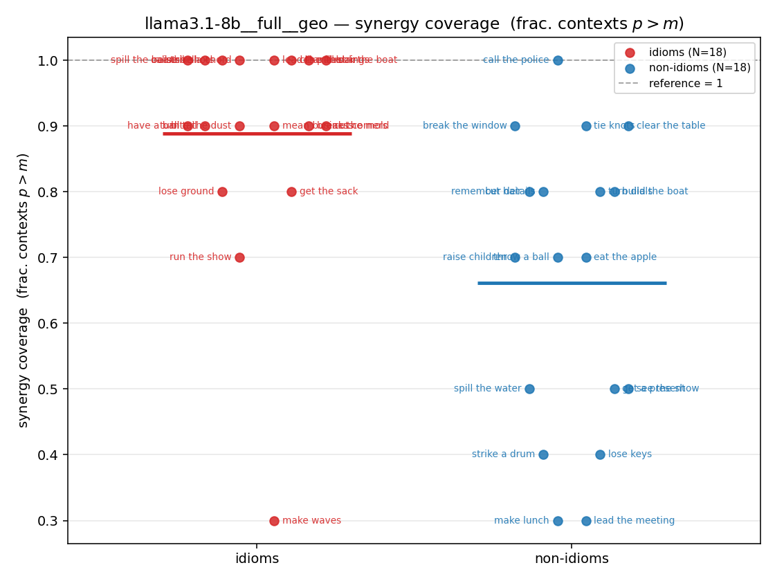 |
| mean ± 95% CI | 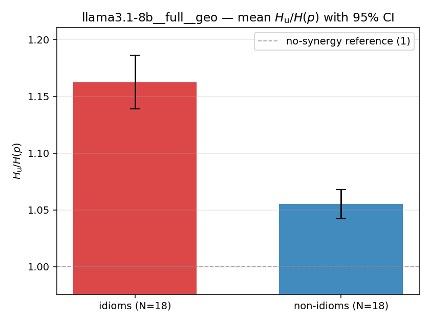 | 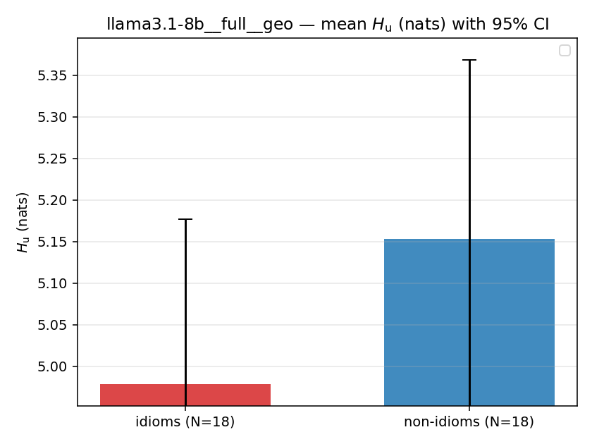 | 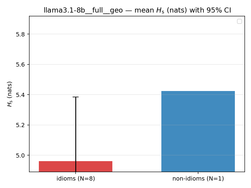 | 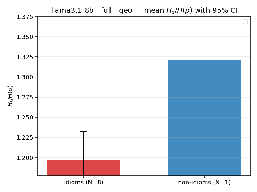 | 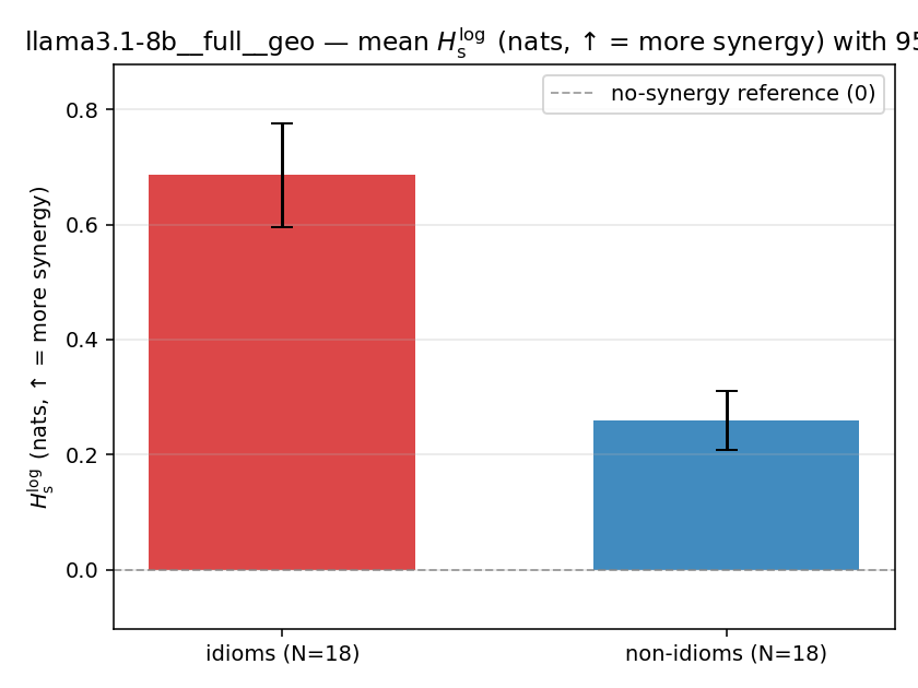 | 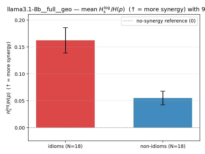 | 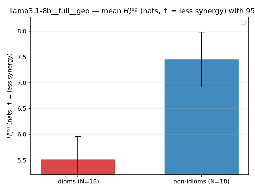 | 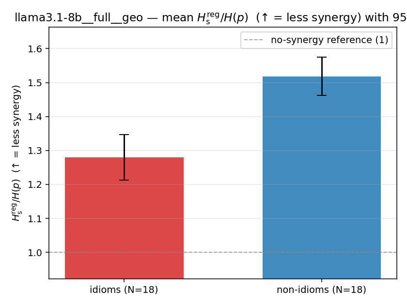 | 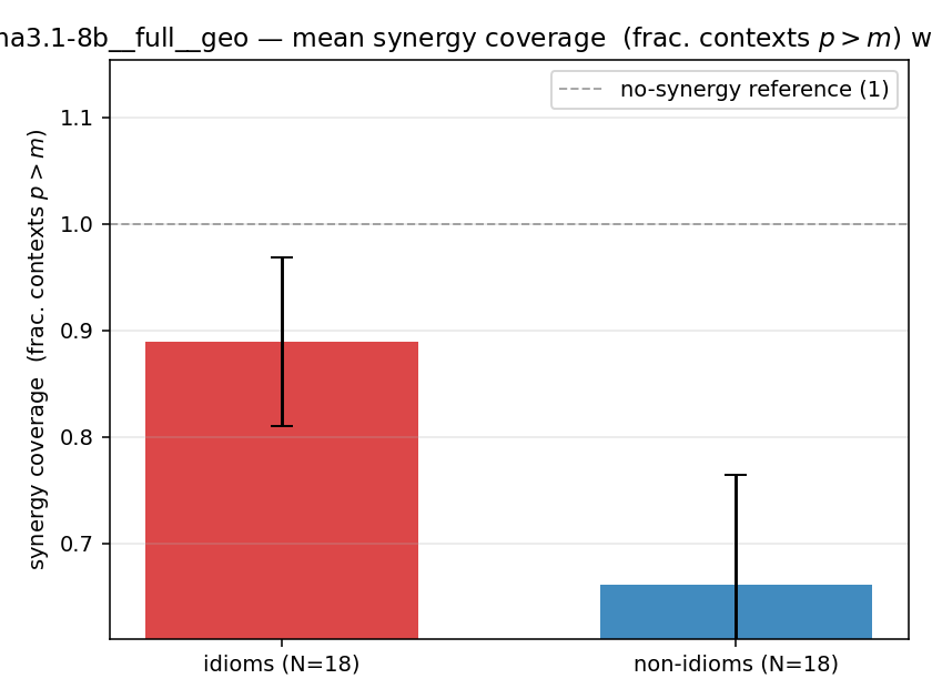 |
| per-idiom (sorted) | 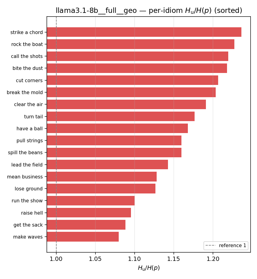 | 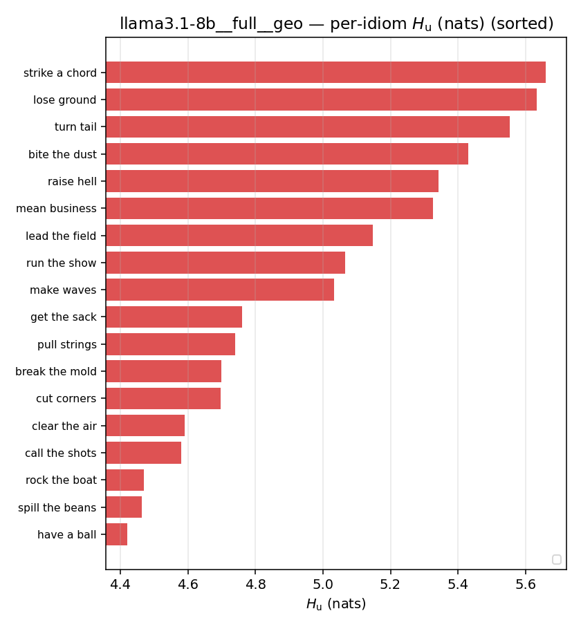 | 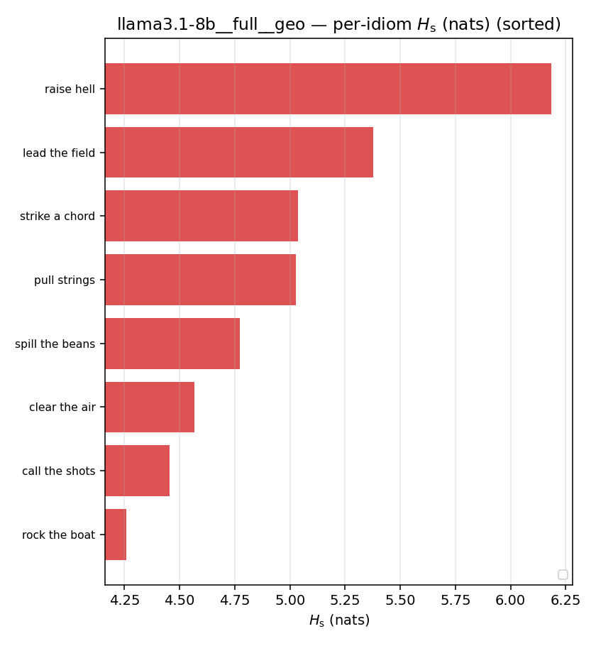 | 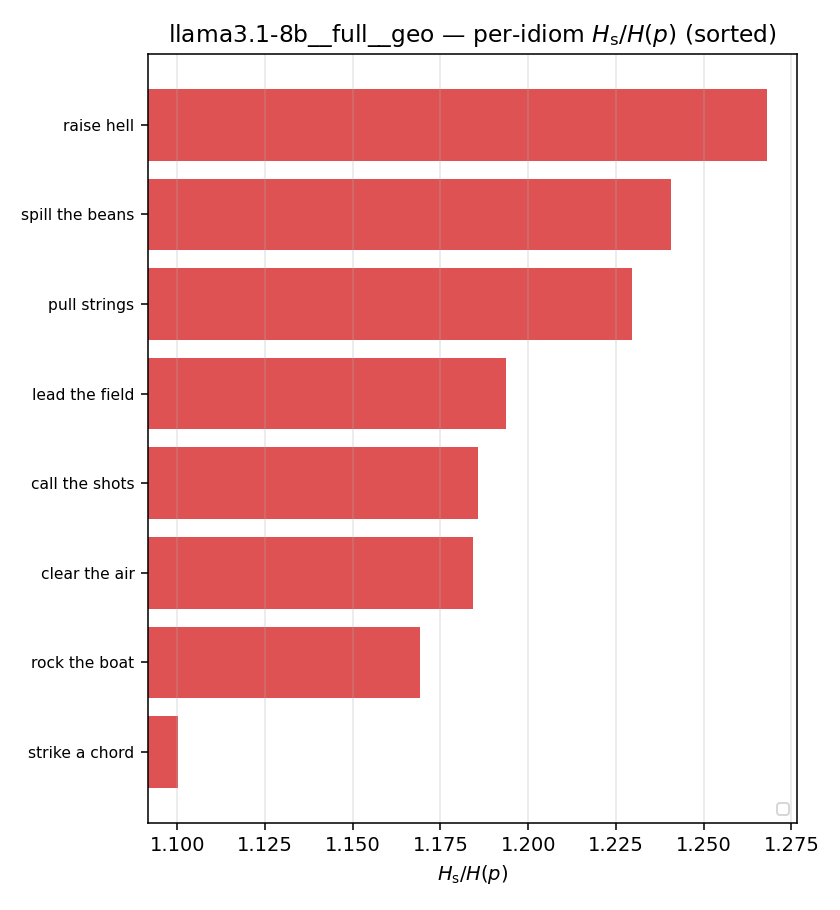 | 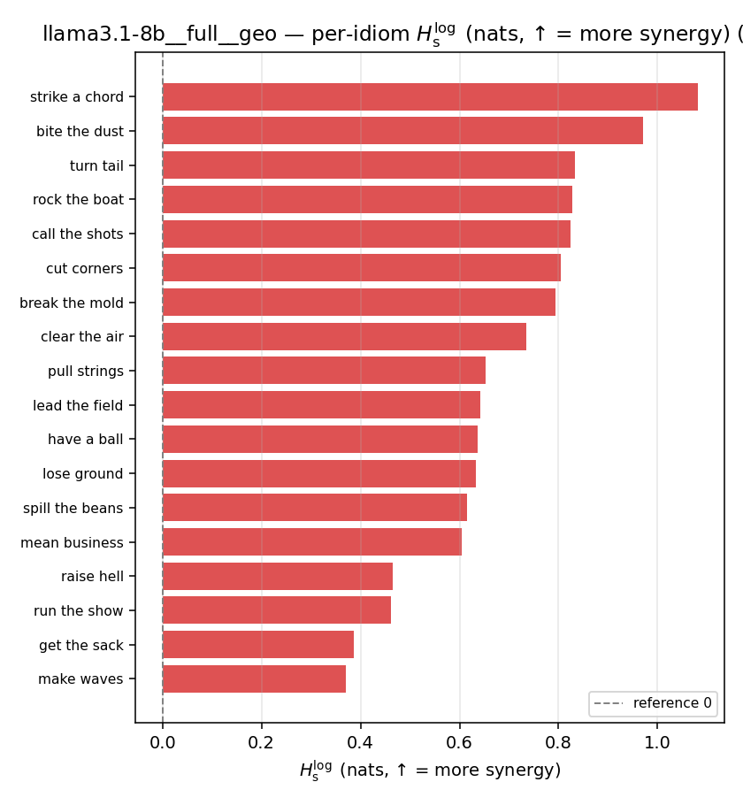 | 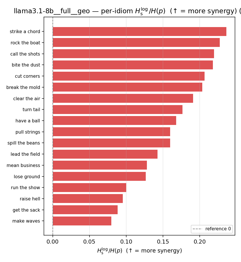 | 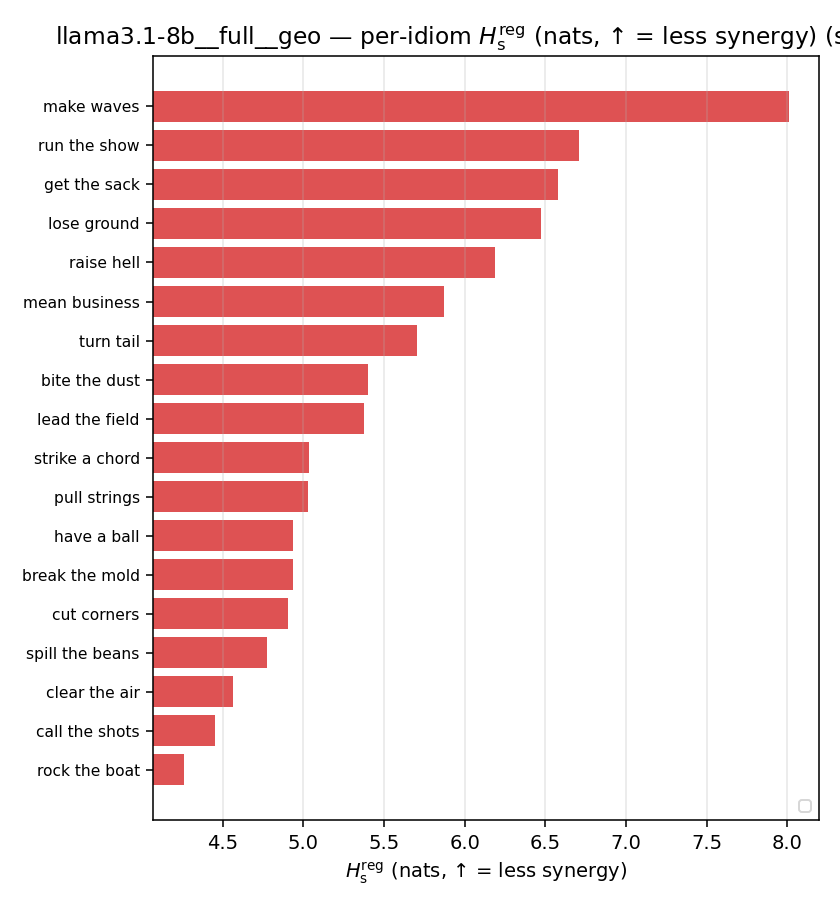 | 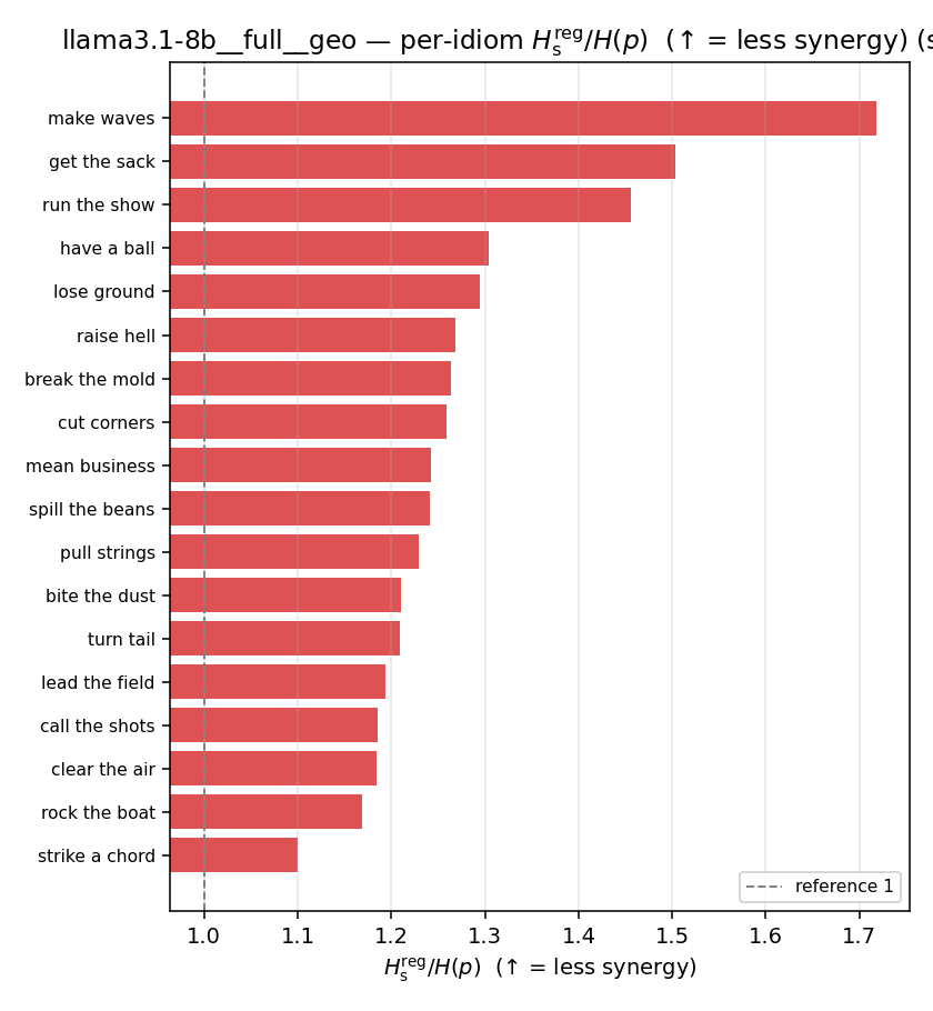 | 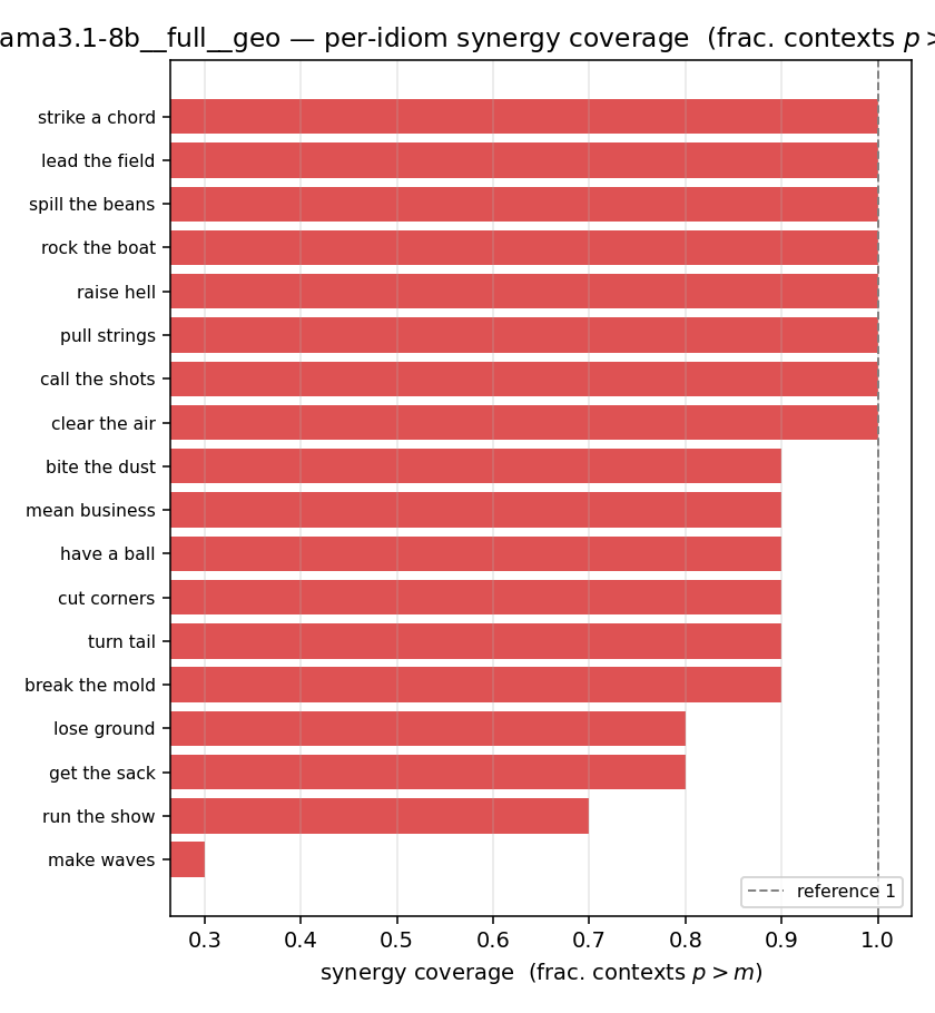 |
llama3.1-8b · full · joint llama3.1-8b__full__joint
| Ĥu/Ĥ ↑syn | Ĥu | Ĥs ↓syn | Ĥs/Ĥ ↓syn | Ĥslog ↑syn | Ĥslog/Ĥ ↑syn | Ĥsreg ↓syn | Ĥsreg/Ĥ ↓syn | f̂syn ↑syn | |
|---|---|---|---|---|---|---|---|---|---|
| strip (per-phrase) | 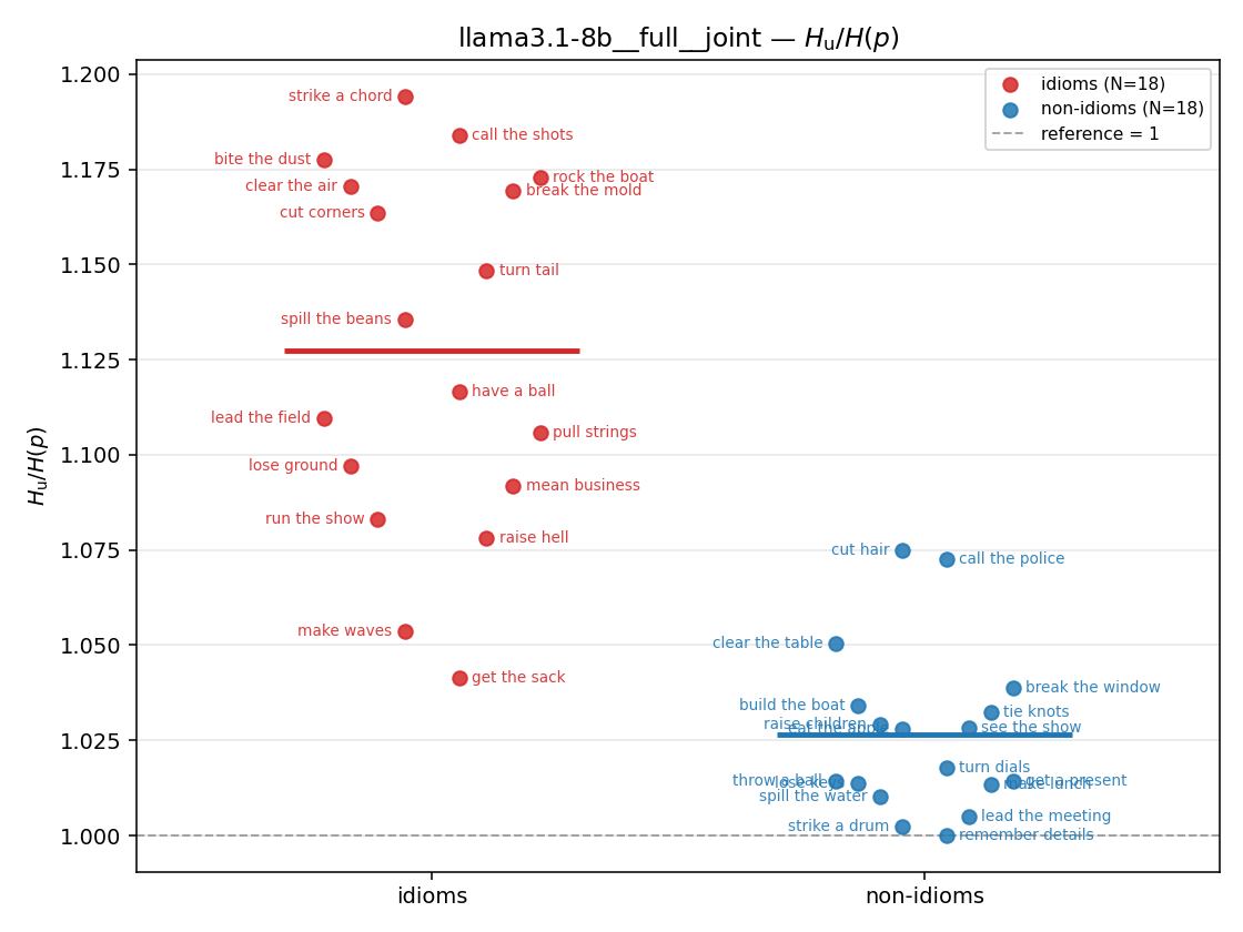 | 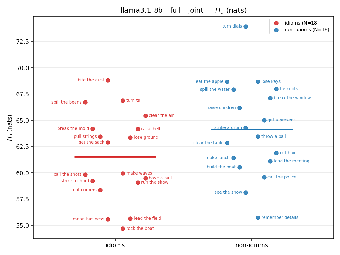 | 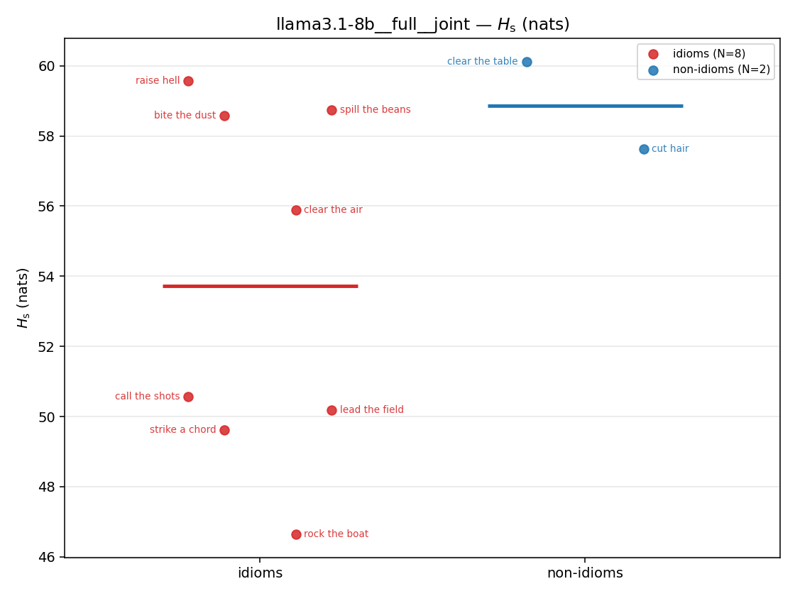 | 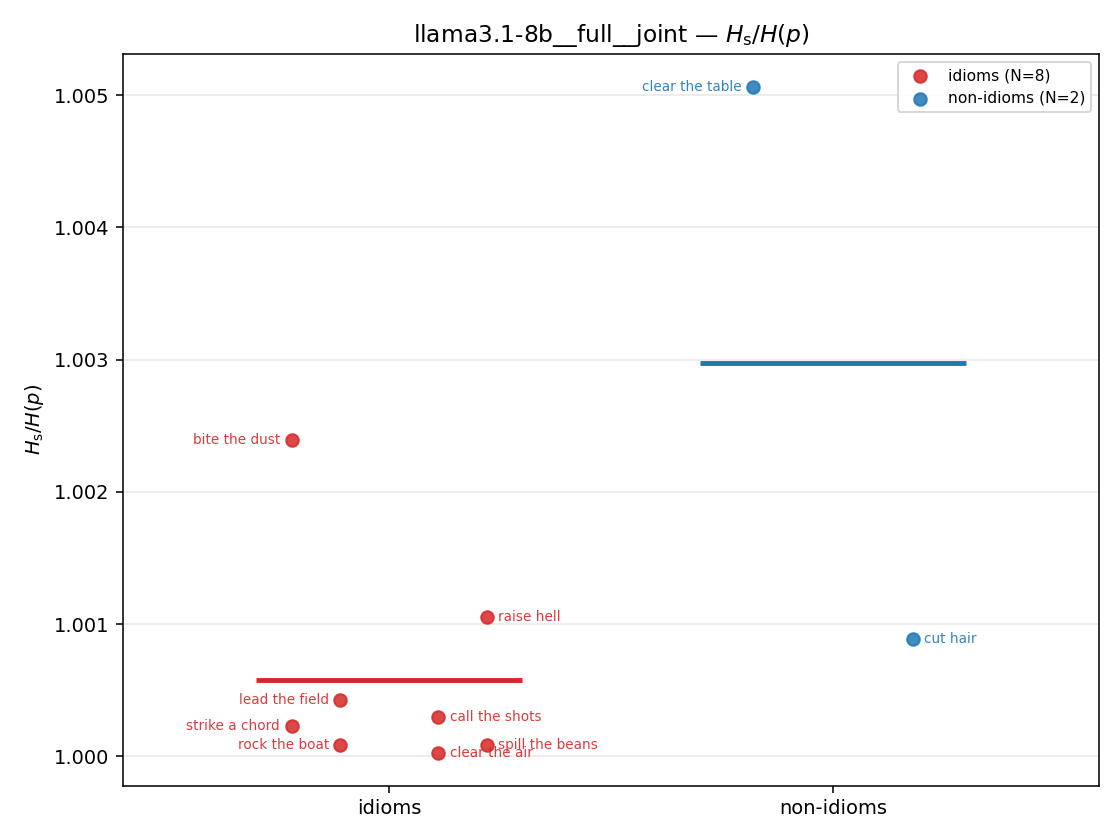 | 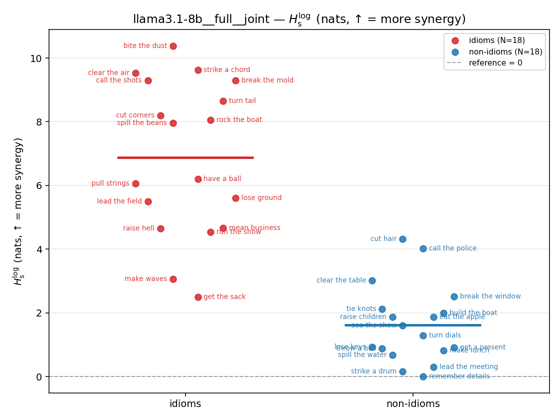 | 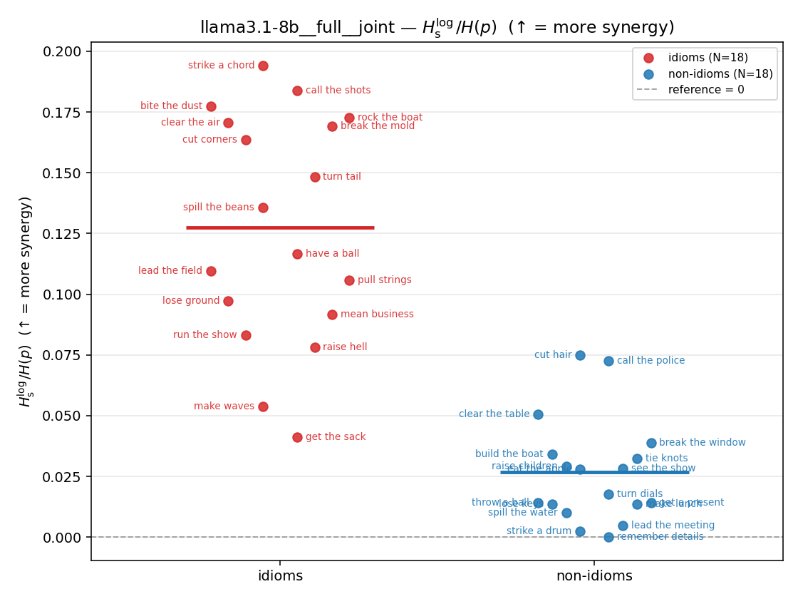 | 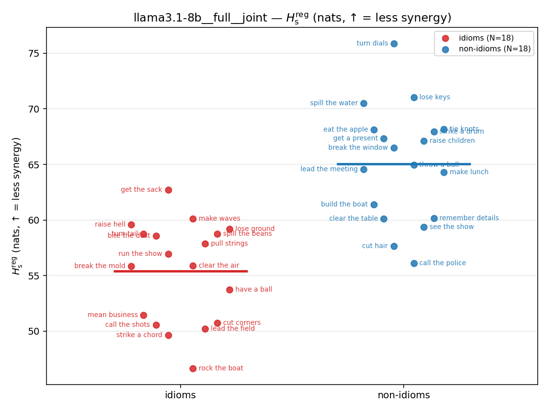 | 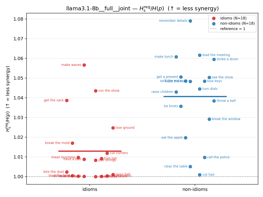 | 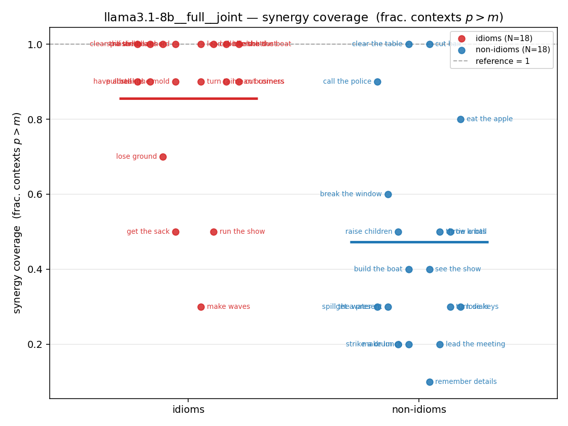 |
| mean ± 95% CI | 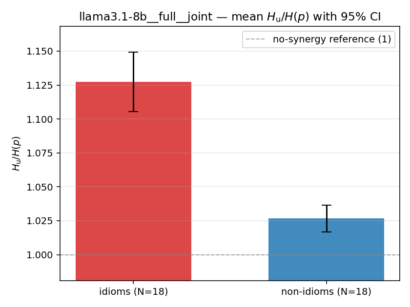 | 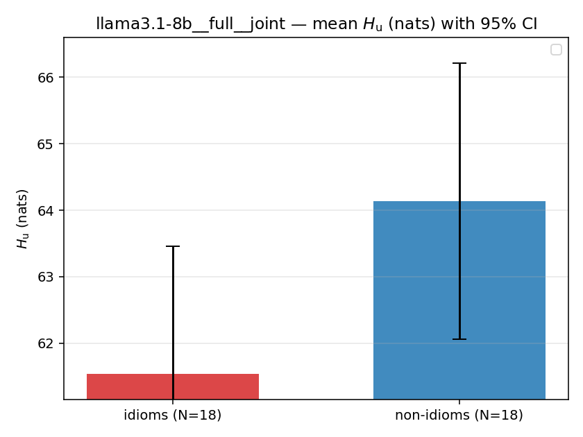 | 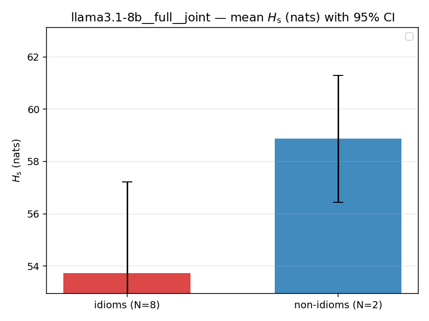 | 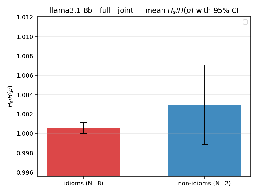 | 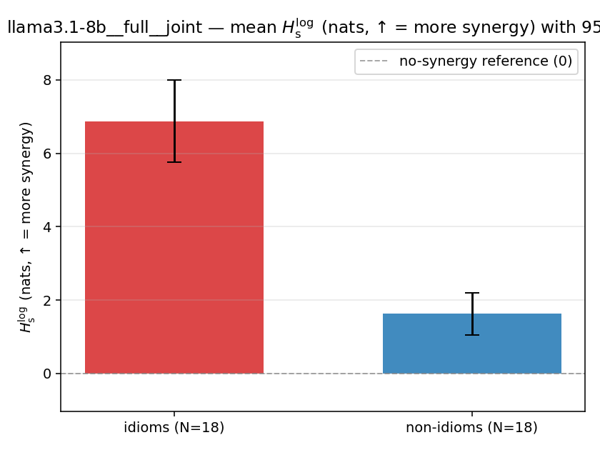 | 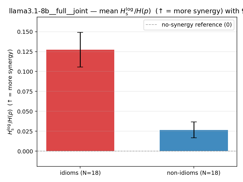 | 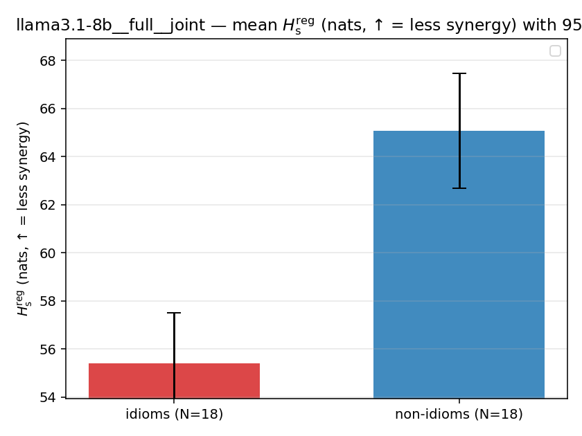 | 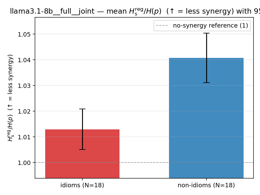 | 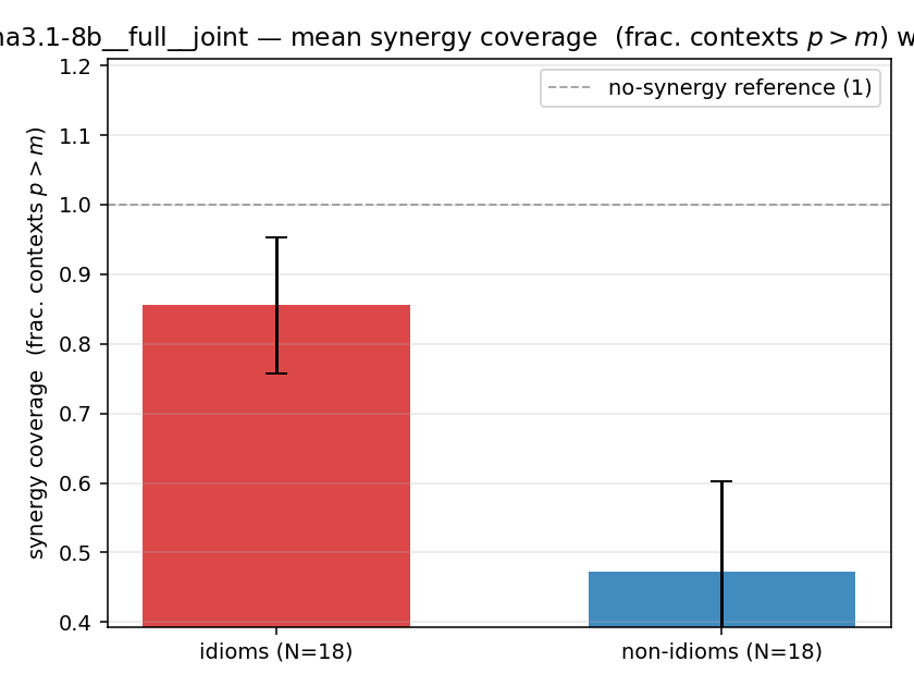 |
| per-idiom (sorted) | 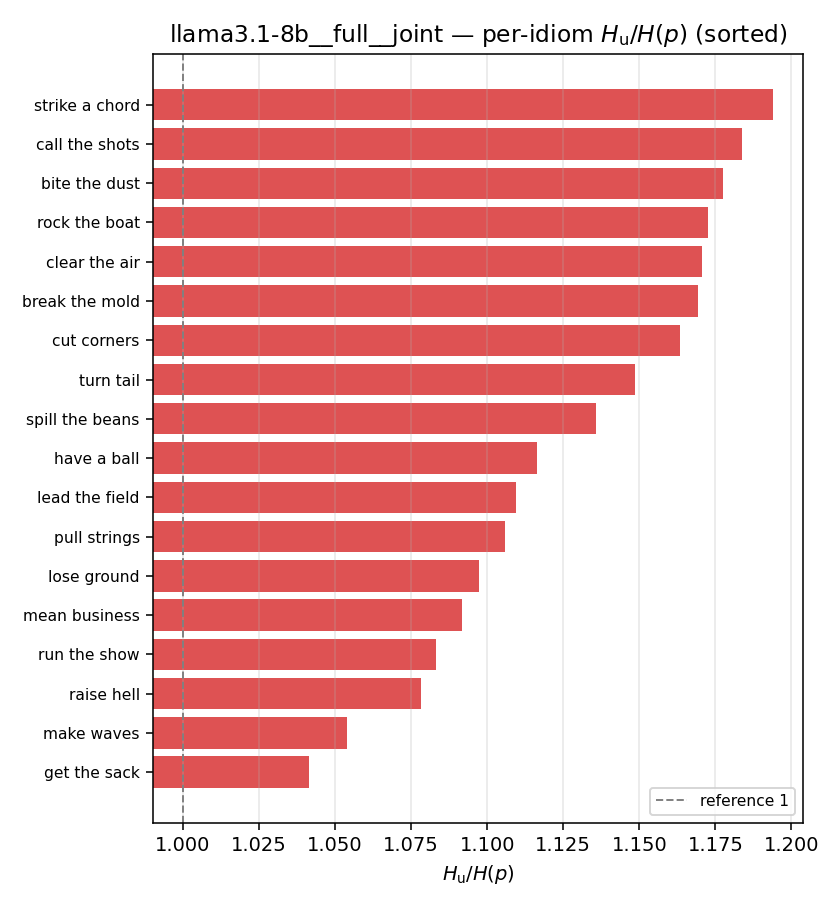 | 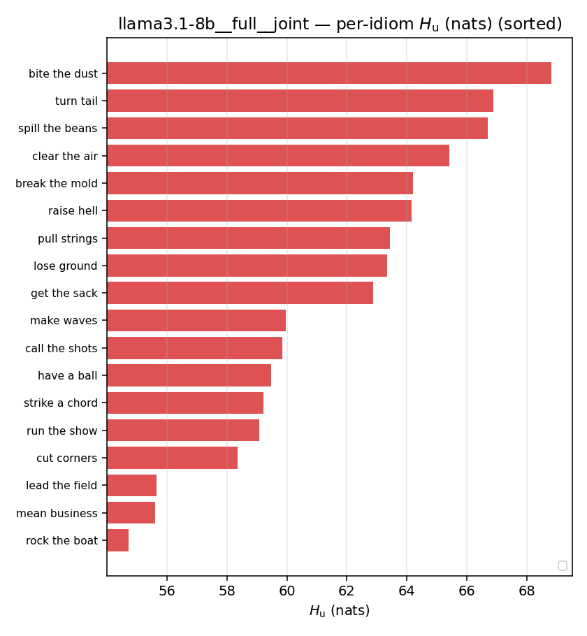 | 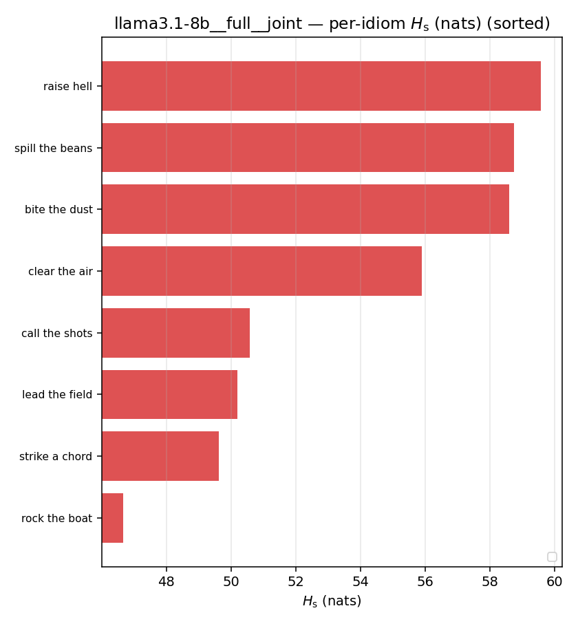 | 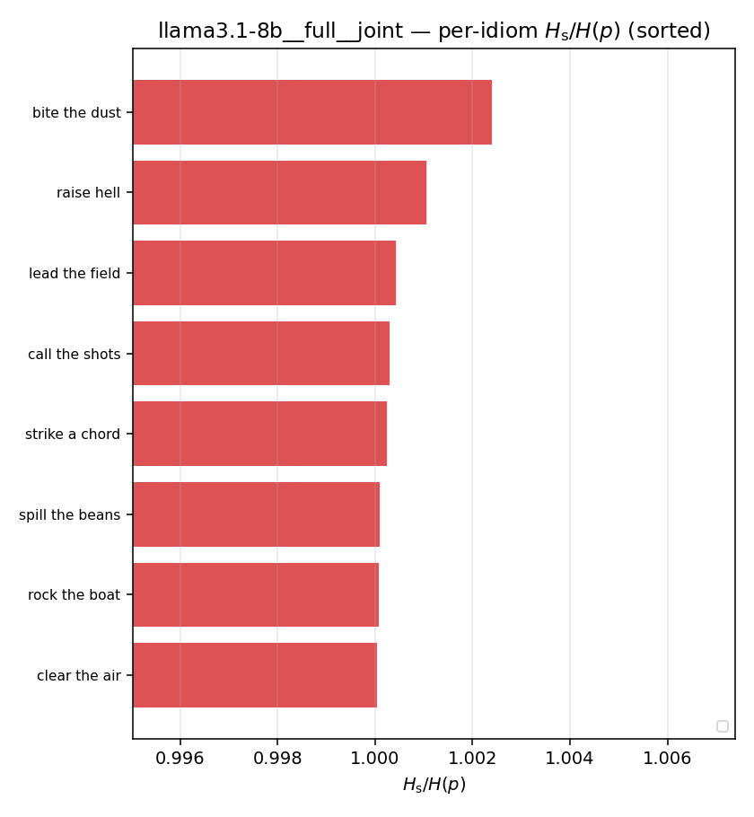 | 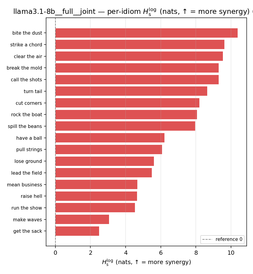 | 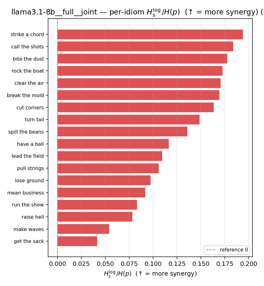 | 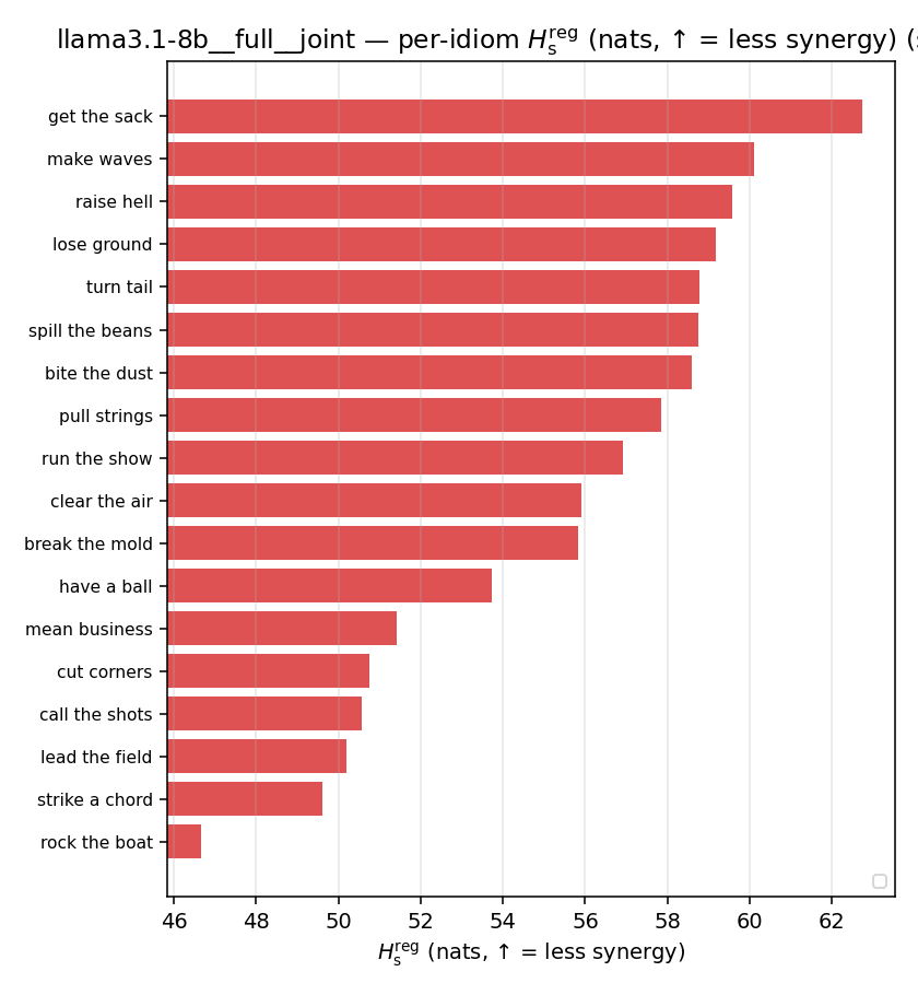 | 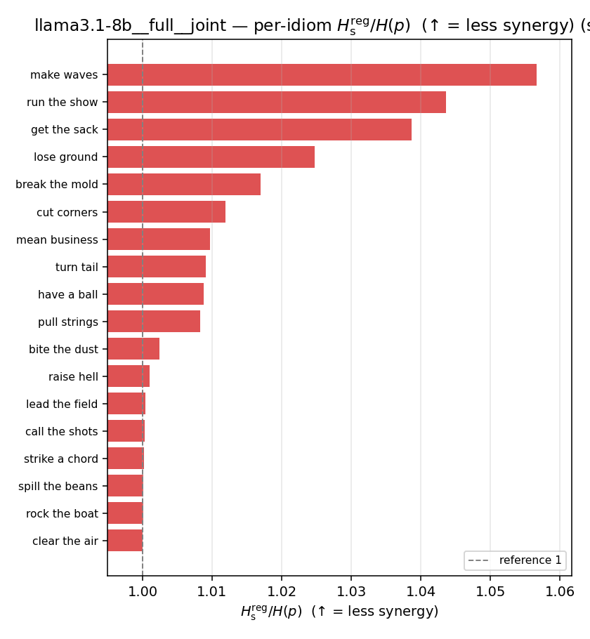 | 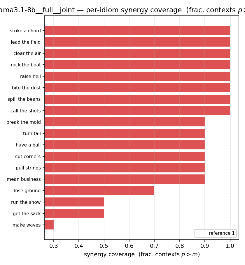 |